Samples, Populations, and Statistical Inference

1. Population vs. Sample: The Ideal and the Real

In statistics, these two terms have precise meanings. Let's start with clear definitions.

To place this in our context:

• Population: This is the entire group we want to draw conclusions about. In finance, the "population" is often a conceptual one. It could be all possible daily returns a crypto asset could ever generate, as described by the true underlying stochastic process we discussed in the last lesson. It is infinitely large and includes the future, making it impossible to observe directly.

• Sample: This is the specific group from which you collect data. For us, a sample is the historical data we can download, for example, the daily closing prices of BTC/USDT from Binance for the last five years. It's a finite, concrete subset of the population.

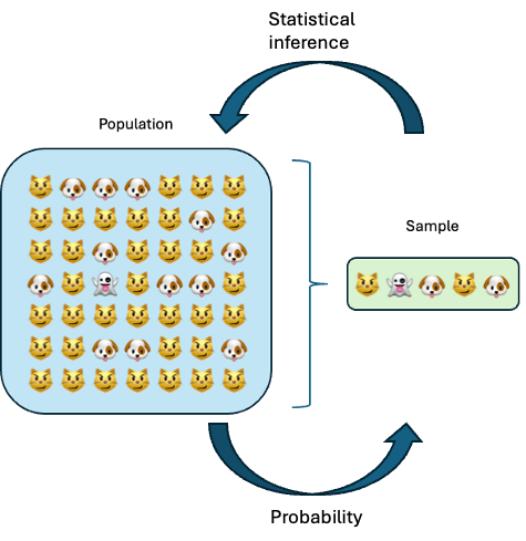
The main reason we use samples is necessity and practicality. It is simply impossible to collect data on every potential outcome. Your experience designing and managing large-scale data systems will make it clear that even if we could access an infinite data stream, processing it would be computationally intractable. We must work with manageable datasets.

2. Describing the Ideal and the Real: Parameters and Statistics

When we measure a characteristic of a population or a sample, we use different terms. This distinction is critical.

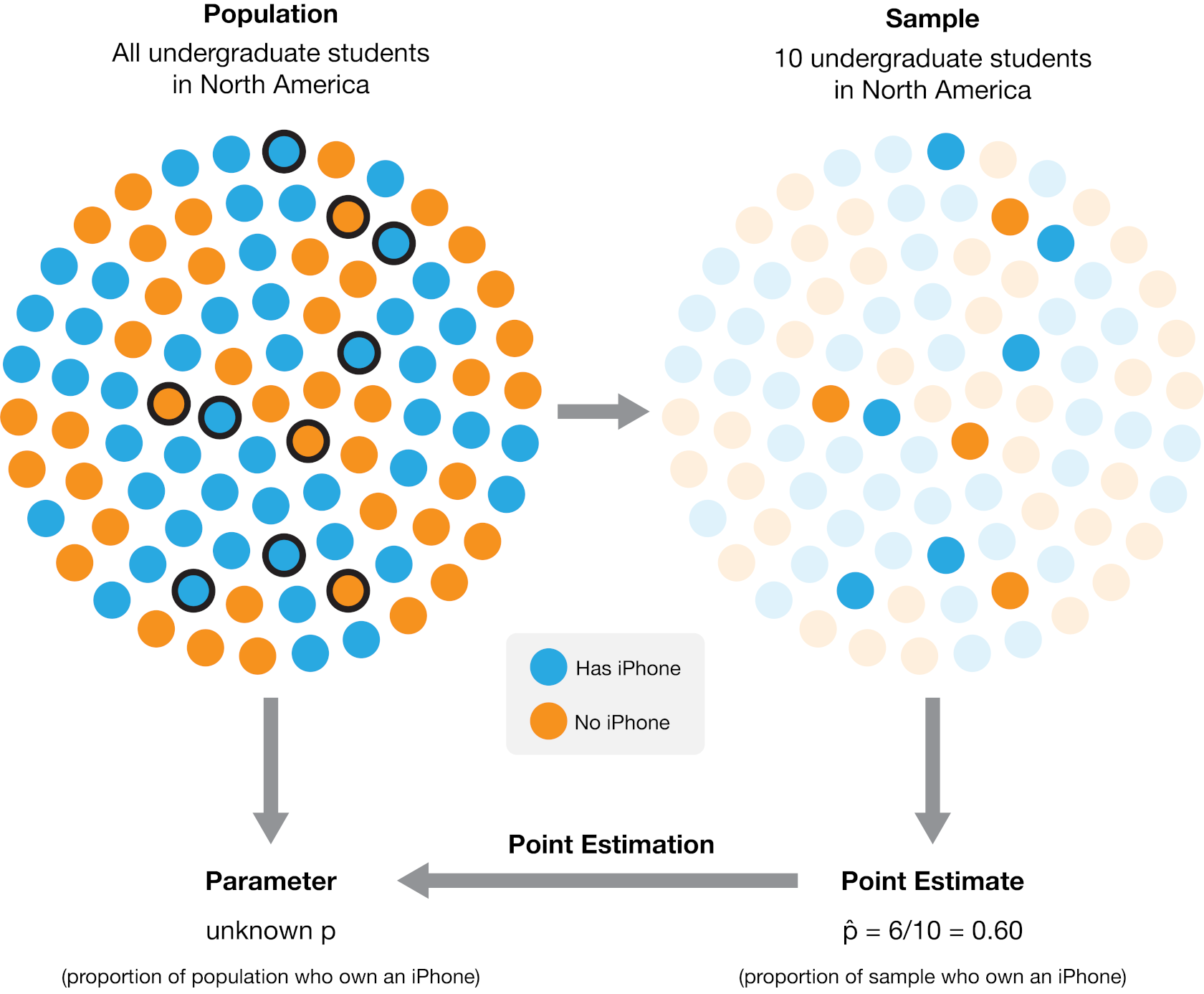
• A Parameter is a value that describes a characteristic of a population. For example, the true mean return ($\mu$) or true volatility ($\sigma$) of an asset are parameters. We can model them, but we can never know their exact values.
• A Statistic is a value that describes a characteristic of a sample. The average return ($\bar{x}$) or standard deviation ($s$) that we calculate from our historical data are statistics.

We use sample statistics as estimates of the true population parameters.

The following video clip clarifies this distinction in a financial context.

So, when we use the Arithmetic Brownian Motion model from our last lesson, $d{S}_t=\mu dt+\sigma d{W}_t$, the $\mu$ and $\sigma$ are population parameters. When you download a year's worth of price data and calculate the mean and standard deviation of daily returns, you are calculating sample statistics—your best guess for the true $\mu$ and $\sigma$.

3. Statistical Inference: The Bridge of Logic

You now know we have a sample, and we want to know about the population. How do we bridge this gap? The answer is statistical inference.

Statistical Inference is the process of using data from a sample to draw conclusions or make predictions about a population.

This is the very essence of quantitative trading. We don't analyze historical data just for fun; we do it to infer something about the future behavior of an asset or a strategy.

Sampling Error: The Unavoidable Gap

As the article mentions, a crucial concept in inference is sampling error. This is the difference between a sample statistic and the true population parameter. It doesn't mean you made a mistake; it's a natural consequence of not observing the entire population.

For example, your backtest on five years of data might show a strategy has an average annual return of 15% (a sample statistic). But its true, long-run average return (the population parameter) might be only 10%. The 5% difference is the sampling error. A central goal in quantitative analysis is to understand and manage this error. You can reduce it by increasing your sample size, but you can never eliminate it.

4. The Importance of a Good Sample

Statistical inference is only reliable if the sample is a good representation of the population. A non-representative, or biased, sample can lead to dangerously wrong conclusions.

For example, imagine you are testing a stock trading strategy. If your sample of stocks only includes companies that are successful and still exist today, you are ignoring all the companies that went bankrupt. This is called survivorship bias. Your sample is not representative of the whole population of stocks that existed over your test period. Consequently, your strategy's performance will appear much better in your backtest than it would in reality.

We will dive much deeper into specific biases like this in Module 5, but for now, it's important to recognize that the quality of the sample is just as important as the analysis you perform on it.

Conclusion

This lesson wraps up our module on the foundations of probability and statistics. We've built a strong conceptual base, moving from descriptive stats to the dynamic world of stochastic processes, and now to the practical realities of working with data.

Key Takeaways:

• A population is the complete set of all possible data points you are interested in (e.g., all future returns of an asset), while a sample is a finite subset of that data you actually have (e.g., historical returns).
• A parameter describes a population (e.g., true mean $\mu$), whereas a statistic describes a sample (e.g., sample mean $\bar{x}$).
• Statistical inference is the formal process of using sample statistics to make educated guesses about population parameters. This is the foundation of data-driven decision-making.
• Sampling error is the inevitable difference between a sample statistic and the population parameter. A key part of a quant's job is to manage this uncertainty.

Preview of the Next Module:

We have now covered the 'why' and 'what' of basic statistical analysis. We understand that we need to compute statistics from samples to infer properties about populations. In our next module, The Quant's Toolkit: Python for Finance, we will begin learning 'how'.

Our very first lesson will introduce NumPy, the workhorse of numerical computing in Python. You'll learn how to perform fast, vectorized operations on arrays of data. These operations are the building blocks for calculating the very sample statistics (like mean, variance, and correlation) we've been discussing, setting the stage for you to start analyzing financial data programmatically.