Assessing Non-Normality with QQ Plots

What is a Quantile-Quantile Plot?

At its core, a Quantile-Quantile (QQ) plot is a graphical method for comparing two probability distributions by plotting their quantiles against each other. For our purposes, we'll compare the quantiles of our sample data (the stock's log returns) against the theoretical quantiles of a perfect normal distribution.

If you're wondering what a quantile is, think of it as a cut-off point that partitions the data. For instance, the 0.5 quantile is the median—50% of the data falls below it. The 0.25 quantile (or 25th percentile) marks the point where 25% of the data falls below it.

To build an intuitive understanding of how a QQ plot is constructed from these quantiles, let's watch a classic explanation from StatQuest.

As the video explains, the power of the QQ plot lies in its simplicity: a straight line indicates a good match, while deviations from that line signal a mismatch between your data's distribution and the theoretical one. Now, let's learn to read those deviations.

Interpreting the Patterns: Skewness and Fat Tails

Deviations from the straight reference line on a QQ plot are not random; they follow distinct patterns that reveal how our data's distribution differs from the normal distribution. For financial returns, we are primarily looking for two things: skewness and kurtosis (fat tails).

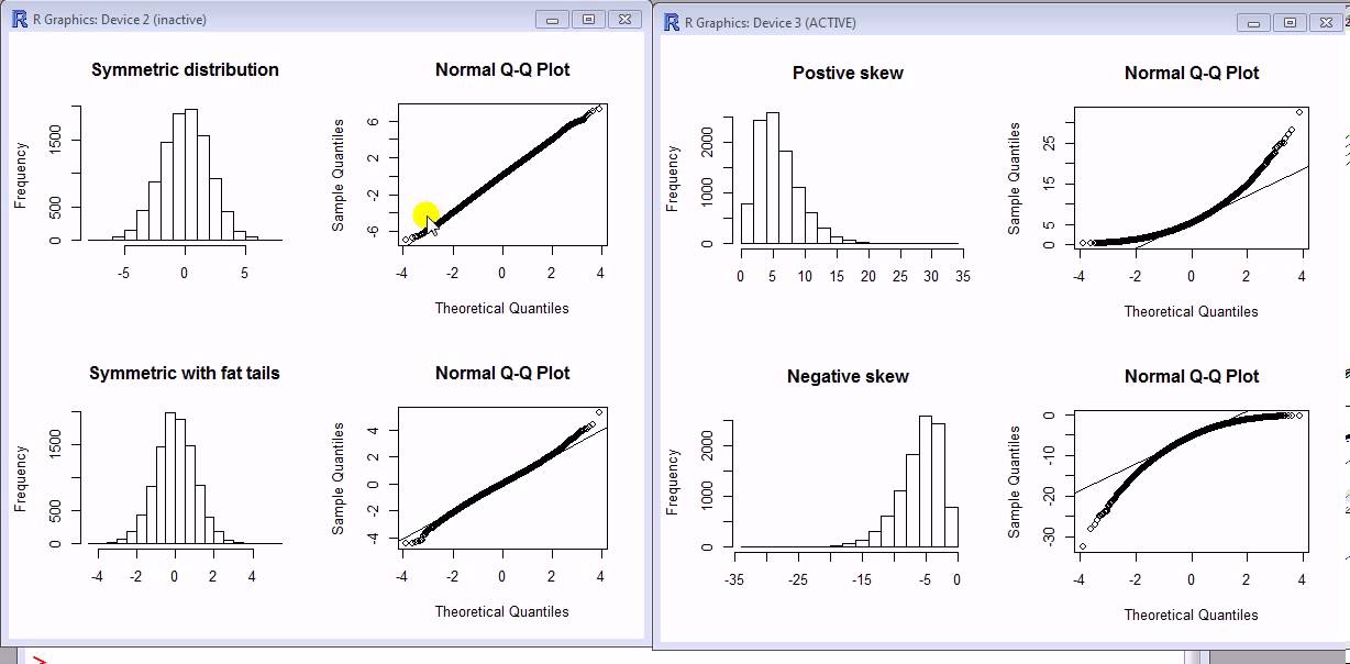
• Fat Tails (Leptokurtosis): This is the most critical pattern for risk management. It appears as an 'S' shape on the QQ plot. The points are below the reference line for low values (left tail) and above the line for high values (right tail). This means your data has more extreme outcomes—both large losses and large gains—than a normal distribution would predict.
• Thin Tails (Platykurtosis): The opposite of fat tails, this forms a reverse 'S' shape. It indicates fewer extreme events than a normal distribution. This is rare for financial returns.
• Right Skew (Positive Skewness): The points form a 'U' shape, consistently staying below the reference line. This indicates that the right tail of your data's distribution is longer than the left.
• Left Skew (Negative Skewness): The points form an inverted 'U' shape, consistently staying above the reference line. This suggests the left tail is longer, which is common in financial returns, reflecting that large crashes can be more frequent or severe than large rallies.

The image below provides a clear visual summary, showing the histogram of a distribution next to its corresponding normal QQ plot for several common cases.

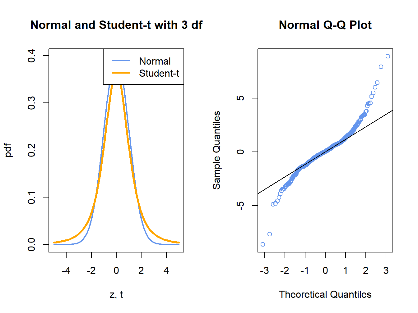
To solidify the "fat tail" signature, consider the following plot. It compares a standard normal distribution to a Student's t-distribution with 3 degrees of freedom—a classic example of a fat-tailed distribution. The QQ plot on the right shows the characteristic 'S' shape, indicating that the tails of the t-distribution are much heavier than those of the normal distribution.

For a more detailed walkthrough of these interpretations, the following resource provides excellent diagrams and explanations.

Practical Application: Generating a QQ Plot in Python

Now let's put this into practice. Your goal for the competition is to build a reusable toolkit, and a function to generate and display a QQ plot is a fundamental component for any data exploration phase.

The video below demonstrates how to compute log returns and then generate a QQ plot using Python's scipy library. It directly applies the concepts we've discussed to real financial data.

To add this to your toolkit, you can use a simple function based on the statsmodels library, which provides a clean and well-annotated plot.

Here is a Python code snippet you can adapt. It takes a pandas Series of returns and generates a QQ plot against a normal distribution.

import numpy as np
import pandas as pd
import statsmodels.api as sm
import matplotlib.pyplot as plt

def plot_qq(returns_series: pd.Series, title: str = "QQ Plot"):
    """
    Generates a Quantile-Quantile plot for a given series of returns
    against a standard normal distribution.

    Args:
        returns_series (pd.Series): A pandas Series of financial returns.
        title (str): The title for the plot.
    """



    # Create the QQ plot
    # 's' is for standardized line (subtract mean, divide by std dev)
    # 'q' is for a line fitted to the quantiles
    # '45' is the 45-degree line
    fig = sm.qqplot(returns_series, line='s', fit=True)
    



    # Customize the plot
    plt.title(title)
    plt.xlabel("Theoretical Quantiles (Normal Distribution)")
    plt.ylabel("Sample Quantiles (Log Returns)")
    plt.grid(True, linestyle='--', alpha=0.6)
    plt.show()




# Example usage:
# Assuming you have a pandas Series `log_returns`
# plot_qq(log_returns, title="QQ Plot of MSFT Log Returns")

This function is a practical asset. During the competition, when you receive a new dataset, one of your first steps should be to calculate log returns and run this function to visually inspect their distribution.

A Deeper Connection: QQ Plots and Kurtosis

Finally, it's worth noting the direct mathematical relationship between the visual pattern of a QQ plot and the statistical measure of kurtosis we discussed in the last lesson. Excess kurtosis (a measure of how fat the tails are) is not about the "peak" of the distribution, but almost entirely about the tails.

An insightful explanation on the same Stack Exchange page clarifies this connection.

Conclusion

In this lesson, we dissected the QQ plot, a fundamental tool for any quantitative analyst. You've learned not only what it is and how to create one in Python, but more importantly, how to interpret its patterns to diagnose the critical properties of financial data.

Here are the key takeaways:

1. Purpose: A QQ plot visually compares your data's quantiles to those of a theoretical distribution (like the normal distribution).
2. Interpretation: A straight line means your data fits the theoretical distribution. Deviations signal a mismatch. For financial returns, the most common pattern is an S-shape, which is the unmistakable signature of fat tails (leptokurtosis).
3. Practical Tool: You now have a reusable Python function to quickly generate a QQ plot for any return series, allowing you to rapidly assess one of the most important stylized facts for any asset.

With this lesson, we conclude our foundational module on financial data and its properties. You are now equipped to describe, process, and diagnose the key statistical features of the data you'll encounter in the competition.

In our next lesson, we will begin Module 2, "Signal Identification & Alpha Research." Building directly on the concept of volatility clustering, you will implement your first feature engineering function: a tool to compute and visualize rolling volatility. This marks our transition from understanding data to actively engineering features for predictive models.