Large Neighborhood Search with Constraint Programming for Solution Repair and Improvement

The LNS "Destroy and Repair" Loop

Let's begin by recapping the overall structure of an LNS algorithm. It's an iterative process that systematically destroys a part of a solution and then intelligently repairs it, seeking improvements at each step.

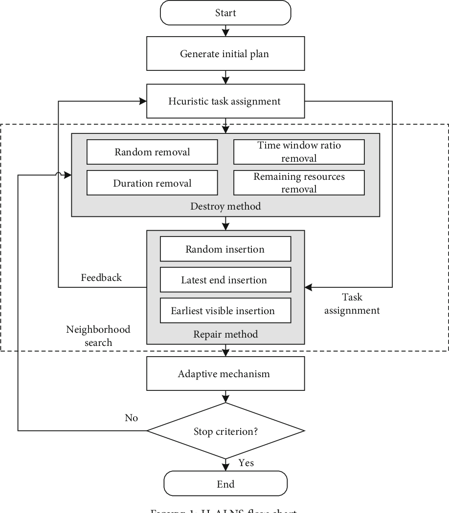
This "destroy and repair" (or "ruin and recreate") cycle is the engine of the LNS metaheuristic. Let's formalize this into an algorithm that you can implement.

The Core LNS-CP Algorithm

The general algorithm for an LNS framework that uses CP as its repair mechanism is straightforward. We can model it based on the state-of-the-art approaches used in academic research.

To start, let's watch a brief segment of the video from our last lesson to refresh our memory of the LNS process.

Now, let's translate this into a concrete algorithmic structure. A great reference is Algorithm 1 from the paper "A unified solution framework for flexible job shop scheduling..." by Kasapidis et al., which we studied in the last lesson. We will adapt and simplify it into a foundational LNS framework.

Here is the pseudocode for your core LNS loop:

Function LNS_CP_Solver(problem_instance, time_limit):
    1.  // Initialization
    2.  start_time = CurrentTime()
    3.  s_best = FindInitialSolution(problem_instance, time_limit_initial)
    4.  s_current = s_best
    5.  
    6.  // Main Loop
    7.  WHILE (CurrentTime() - start_time < time_limit):
    8.      // 1. Ruin Phase: Select operator and destroy part of the solution
    9.      destroy_operator = SelectDestroyOperator()
    10.     partial_solution = destroy_operator.apply(s_current)
    11.     fixing_constraints = GenerateFixingConstraints(partial_solution)
    12.     
    13.     // 2. Repair Phase: Use CP to find a new solution
    14.     s_new = CPSolve(problem_instance, fixing_constraints, time_limit_per_iteration)
    15.     
    16.     // 3. Acceptance Phase
    17.     IF Objective(s_new) < Objective(s_current):
    18.         s_current = s_new
    19.         IF Objective(s_new) < Objective(s_best):
    20.             s_best = s_new
    21.             print("New best solution found:", Objective(s_best))
    22.
    23. RETURN s_best

Let's break down each part:

• Initialization (Lines 2-4): You start by finding an initial feasible solution. This is typically done by running your base CP model with a short time limit. This solution, s_best, is your initial benchmark.
• Main Loop (Line 7): The search continues until a global stopping criterion is met, like a total time budget.
• Ruin Phase (Lines 9-11): At each iteration, you select a "destroy" operator. This operator takes the current solution s_current and decides which parts to "free up". The output is essentially a set of fixing_constraints that lock down the parts of the solution you didn't destroy.
• Repair Phase (Line 14): This is the call to your CP solver. You solve the original problem model, but you add the fixing_constraints. Crucially, this call has its own, much shorter, time limit (time_limit_per_iteration). Its job is to find a good completion quickly, not to prove optimality.
• Acceptance Phase (Lines 17-21): This is the simplest acceptance criterion: only accept improvements (a "greedy" approach). If the new solution s_new is better than s_current, you accept it. If it's also the best seen so far, you update s_best.

Implementing the Destruction Operators

The real art of LNS lies in the implementation of the destruction operators. Their goal is to define a "neighborhood" of the current solution to be explored by the CP solver. A good operator generates subproblems that are both small enough to be solved quickly and promising enough to contain better solutions.

The paper "Large Neighborhood Search and Adaptive Randomized Decompositions for Flexible Jobshop Scheduling" provides very clear definitions that are perfect for a first implementation.

Based on what you've read, let's outline how to implement these three fundamental operators. In each case, the operator must perform two tasks:

1. Select a set of operations to "free," let's call this set $O_{free}$.
2. Generate fixing constraints for all other operations, $O_{fixed}=\Omega \setminus O_{free}$, where $\Omega$ is the set of all operations.

1. Random Operator

This operator is the simplest and is great for diversifying the search.

• Logic:
  1. Choose a destruction rate, p (e.g., 0.2 for 20%).
  2. Randomly select p * |Ω| operations and add them to the set $O_{free}$.
• Fixing Constraints: For all operations in $O_{fixed}$.

2. Time-Window Operator

This operator focuses the search on a specific temporal part of the schedule.

• Logic:
  1. Get the makespan C_max of the current solution.
  2. Choose a window size, w (e.g., 0.3 * C_max).
  3. Choose a random start time for the window, t_start, between 0 and C_max - w. The window is [t_start, t_start + w].
  4. Iterate through all operations. An operation i is added to $O_{free}$ if its schedule in s_current overlaps with the window (i.e., start_time(i) < t_start + w and end_time(i) > t_start).
• Fixing Constraints: For all operations in $O_{fixed}$.

3. Machine Operator

This operator focuses on re-optimizing the workload of one or more machines, which is often effective for resolving bottlenecks.

• Logic:
  1. Choose a number of machines to free, k (e.g., 1 or 2).
  2. Randomly select k machines.
  3. Add all operations currently assigned to these k machines in s_current to the set $O_{free}$.
• Fixing Constraints: For all operations in $O_{fixed}$.

Generating the Fixing Constraints

This is the most technical part of the implementation. Based on the concept of a "Fully POS-feasible Solution", for every operation $i\in O_{fixed}$, you must constrain its machine assignment and its relative order with other fixed operations on the same machine.

Here is the pseudocode for the GenerateFixingConstraints function:

Function GenerateFixingConstraints(s_current, O_fixed):
    constraints = []
    
    // 1. Fix machine assignments
    FOR each operation i IN O_fixed:
        assigned_machine = s_current.get_machine(i)
        // This assumes your CP model has a way to enforce an assignment,
        // e.g., by fixing a variable or using PresenceOf().
        constraints.add(ForceAssignment(i, assigned_machine))
        
    // 2. Fix relative sequences on each machine
    machines = GetAllMachines()
    FOR each machine m IN machines:
        // Get the sequence of fixed operations on this machine from s_current
        sequence_on_m = []
        FOR each operation j scheduled on m IN s_current:
            IF j IN O_fixed:
                sequence_on_m.add(j)
        
        // Sort them by their start times in s_current
        sequence_on_m.sort(by=s_current.get_start_time)
        
        // Add precedence constraints for adjacent operations in the sequence
        FOR k from 0 to len(sequence_on_m) - 2:
            op1 = sequence_on_m[k]
            op2 = sequence_on_m[k+1]
            // Add a constraint like EndBeforeStart(op1, op2)
            constraints.add(EnforcePrecedence(op1, op2))
            
    RETURN constraints

Your CPSolve function will then take these constraints and add them to the base model before solving.

Advanced Considerations

While the framework above is a complete and powerful starting point, the research papers we've seen point to more advanced techniques you can integrate as you develop your solver:

• Adaptive Operator Selection: Instead of choosing a destruction operator randomly, you can implement a roulette-wheel selection mechanism that gives more weight to operators that have recently produced better solutions (as described in Kasapidis et al., Section 4.3).
• Memory-based Operators: As seen in the "Machine Assignment Operators" from Kasapidis et al., you can store a pool of "elite" solutions and use the frequency of certain assignments or sequences to guide the destruction process, either by forbidding rare patterns or enforcing common ones.
• Sophisticated Acceptance Criteria: Instead of only accepting better solutions, you can use a criterion from Simulated Annealing that sometimes accepts worse solutions with a certain probability, helping the search escape local optima.

Conclusion

In this lesson, we have laid out a comprehensive, practical blueprint for implementing an LNS-CP hybrid solver for the FJSP.

Key Takeaways:

• The LNS algorithm is an iterative loop of ruining a part of a solution and repairing it with a time-limited CP solver call.
• The "ruin" phase is implemented via destruction operators (e.g., random, time-window, machine-based) that select a subset of operations to free.
• The implementation of these operators involves generating fixing constraints for the unfreed parts of the solution, which typically involves fixing both machine assignments and the relative sequence of operations on each machine.
• This LNS-CP framework provides a robust and high-performance approach that leverages the respective strengths of metaheuristics (broad exploration) and CP (deep, constrained search), making it an excellent choice for your thesis research.

Preview of the Next Module:

You have now completed the modules on modeling and solving complex scheduling problems. You have learned to formulate problems using MILP and CP, model advanced constraints, and design and implement sophisticated hybrid metaheuristics.

The next step is to apply these skills within a rigorous academic framework. Our next module, Research Methodology for Scheduling, will prepare you for this. We will cover how to conduct a thorough literature review, identify research gaps, select appropriate benchmark instances and performance metrics, design and execute computational experiments, and ultimately articulate a clear and defensible contribution for your thesis.