Simulated Annealing: Neighborhood Search & Cooling Schedules

1. The Inspiration: Annealing in Metallurgy

The core idea behind Simulated Annealing is borrowed directly from a process in metallurgy, which, given your background in industrial engineering, should provide a strong intuitive foundation. When a metal is heated to a high temperature, its atoms have a lot of energy and move around freely. If it's cooled very quickly ("quenched"), the atoms get locked into a high-energy, disordered state. However, if it's cooled slowly and carefully—a process called annealing—the atoms have time to settle into a highly ordered, low-energy crystalline structure.

Simulated Annealing applies this same principle to optimization:

• A solution is like the arrangement of atoms in the material.
• The cost of a solution (e.g., makespan) is like the energy of the system.
• The global optimum is the minimum energy state (the perfect crystal).
• Temperature is a control parameter that manages the search process.

To start, let's watch a video that introduces this physical analogy and explains why algorithms like SA are needed to overcome the limitations of simple local search.

This analogy gives us the core strategy of SA: start "hot" to explore the search space widely, and then gradually "cool down" to exploit promising regions and settle on a high-quality solution.

2. The Simulated Annealing Algorithm

At its heart, SA is a modified version of hill climbing. While a simple hill-climbing algorithm only ever accepts moves that improve the solution, SA allows for "bad" moves (moves that worsen the solution) with a certain probability. This ability is what allows it to escape from local optima.

The general structure of the algorithm is as follows:

The algorithm can be summarized in these steps:

1. Initialize:
   • Generate an initial solution, $S_{current}$.
   • Set a high initial temperature, $T$.
2. Loop until a stopping condition is met:
   • For a fixed number of iterations:
     • Generate a neighboring solution, $S_{new}$, from the neighborhood of $S_{current}$.
     • Calculate the change in the objective function: $\Delta f=f(S_{new})-f(S_{current})$. For makespan minimization, this is $\Delta C_{max}$.
     • Decide whether to accept $S_{new}$ using the acceptance criterion (we'll detail this next). If accepted, set $S_{current}=S_{new}$.
   • Cool down: Reduce the temperature $T$ according to a cooling schedule.

The two most critical components of this algorithm are the acceptance criterion and the cooling schedule.

3. The Acceptance Criterion: The Metropolis Rule

How does SA decide whether to accept a worse solution? It uses a probabilistic rule known as the Metropolis criterion.

If the new solution $S_{new}$ is better than the current one $S_{current}$ (i.e., $\Delta f<0$ for minimization), it is always accepted.

If $S_{new}$ is worse (i.e., $\Delta f\ge 0$), it is accepted with a probability given by the Boltzmann distribution:

Let's break down this formula:

• $\Delta f$: The change in cost. The larger the increase in cost (the "worse" the move), the smaller the exponential term becomes, and the lower the acceptance probability.
• $T$: The current temperature.
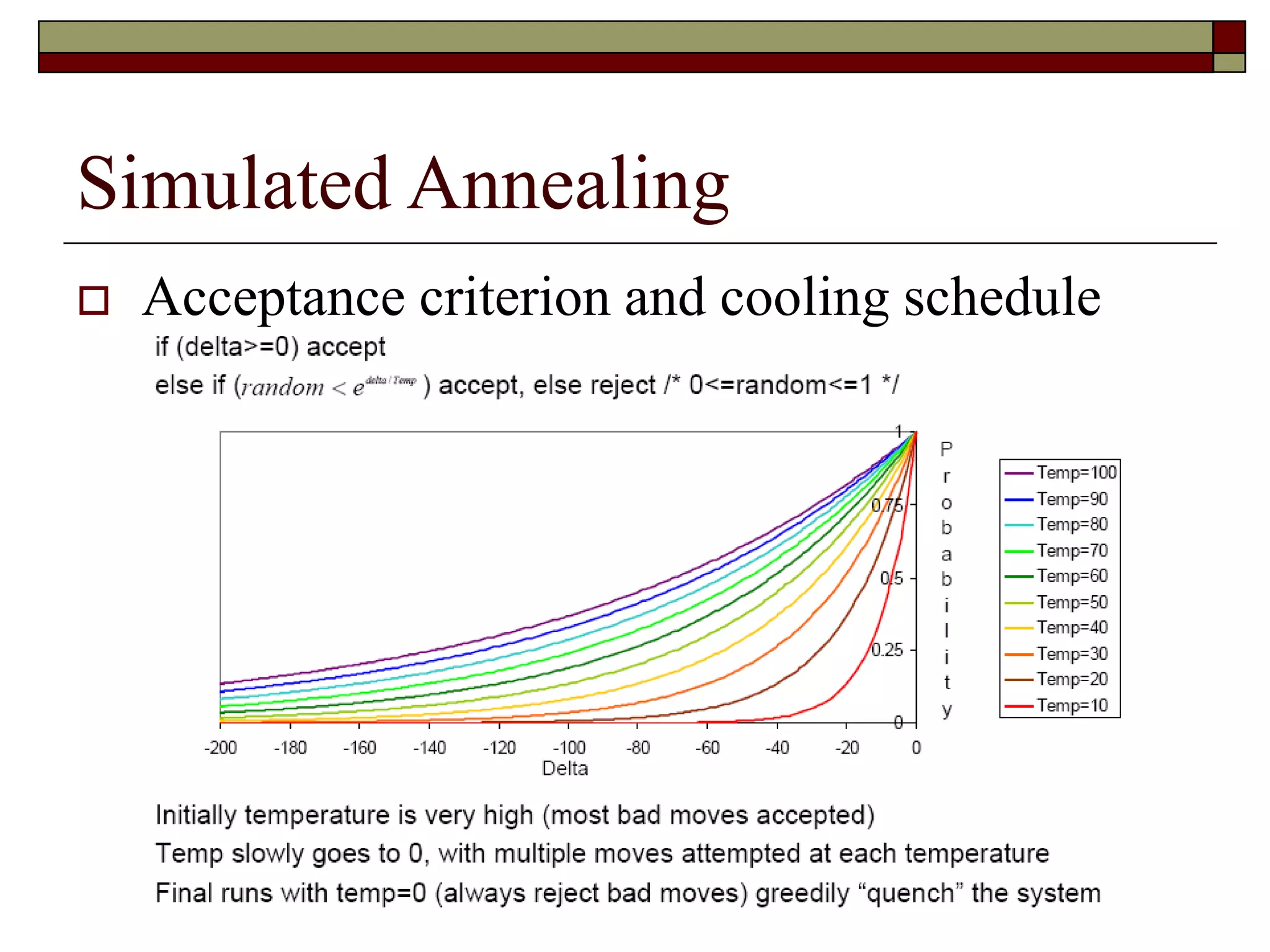
  • When $T$ is high, the fraction $-\frac{\Delta f}{T}$ is close to zero, so $P(\text{accept})$ is close to $\exp (0)=1$. The algorithm accepts almost any move, leading to a random-walk-like exploration.
  • When $T$ is low, the fraction becomes a large negative number, so $P(\text{accept})$ is close to 0. The algorithm is very unlikely to accept bad moves, behaving like a simple hill-climbing algorithm (exploitation).

The following video section provides a brilliant numerical illustration of how this probability changes with both $\Delta f$ and $T$.

The image below provides a great graphical summary of this relationship.

4. The Cooling Schedule

The cooling schedule dictates how the temperature $T$ decreases over time. It is a critical part of the algorithm that controls the balance between exploration and exploitation. A poorly designed schedule can either terminate the search prematurely in a poor-quality region (cooling too fast) or waste computational time exploring randomly (cooling too slow).

A cooling schedule is defined by four key parameters:

Let's summarize these crucial components:

1. Initial Temperature ($T_{init}$): This should be high enough to allow the algorithm to freely explore at the beginning. A common practice is to set $T_{init}$ such that the initial acceptance rate for worsening moves is high (e.g., 80% or more). This can be found by running some trial moves and calculating the required $T_{init}$ based on the average $\Delta f$ of those moves.

2. Cooling Function: This defines how the temperature is reduced. The most common method is geometric cooling:

   $$T_{k+1}=\alpha \cdot T_k$$

   Here, $\alpha$ is the cooling rate, a value typically between 0.8 and 0.99.

   • A value of $\alpha$ close to 1 (e.g., 0.99) results in very slow cooling, allowing for extensive exploration but requiring more computation time.
   • A smaller $\alpha$ (e.g., 0.85) cools much faster, leading to quicker convergence but with a higher risk of getting stuck in a local optimum.

3. Iterations per Temperature Step (Markov Chain Length): At each temperature level, the algorithm runs for a certain number of iterations. This allows the system to reach a "quasi-equilibrium" at that temperature before cooling further. A common choice is a fixed number of iterations, or a number proportional to the size of the problem (e.g., the number of operations).

4. Termination Criterion: The algorithm must have a condition to stop. Common criteria include:

   • The temperature reaches a very low final temperature ($T_{final}$).
   • The best solution found has not improved for a certain number of consecutive temperature steps.
   • A maximum number of iterations or a total runtime limit is reached.

The effectiveness of SA is highly sensitive to the tuning of these parameters, which often requires empirical testing for a specific problem domain.

5. Applying SA to the Flexible Job Shop Problem (FJSP)

To apply SA to your specific problem of interest, FJSP, we need to define the "neighborhood" and the "cost function".

• Cost Function: This is straightforward. For makespan minimization, the cost function $f(S)$ is simply the makespan $C_{max}$ of the schedule $S$.

• Neighborhood Search: This is the mechanism for generating a new solution $S_{new}$ from $S_{current}$. Since an FJSP solution involves both job sequencing and machine assignment, a neighborhood move can alter one or both of these components.

As described in the text, typical neighborhood moves for FJSP include:

• Resequencing: Altering the order of operations on a machine. This can be a simple swap of two operations on the same machine or an insertion of one operation into a different position in the sequence.
• Reassignment: Changing the machine assigned to a particular operation (while respecting the set of machines capable of performing it). This directly addresses the "flexible" part of the FJSP.

By combining these moves, the neighborhood search can effectively explore the vast solution space of both operation sequencing and machine allocation that characterizes the FJSP.

Conclusion

In this lesson, we have dissected the Simulated Annealing algorithm, a cornerstone of metaheuristic optimization. You've seen how its power lies in its probabilistic acceptance of non-improving moves, allowing it to systematically escape local optima.

Key Takeaways:

• Simulated Annealing is a single-solution metaheuristic inspired by the physical annealing process in metallurgy.
• It balances exploration at high temperatures with exploitation at low temperatures.
• The Metropolis acceptance criterion, $P(\text{accept})=\exp (-\Delta f/T)$, is the core mechanism that allows the algorithm to accept "bad" moves, with a probability dependent on the move's quality and the current temperature.
• The cooling schedule (initial temperature, cooling rate, iterations per step, and termination criterion) is critical for guiding the search effectively and must be carefully tuned.
• For scheduling problems like FJSP, neighborhood moves typically involve resequencing operations or reassigning them to different machines.

Preview of the Next Lesson:

We have now seen a population-based approach (GA) and a probabilistic single-solution approach (SA). In our next lesson, we will explore Tabu Search (TS). You will see how TS uses a completely different mechanism to escape local optima: memory. Instead of relying on probability, TS deterministically forbids (makes "tabu") recent moves to prevent cycling and force the search into new, unexplored regions of the solution space.