Resource Modeling with Global Constraints

1. A Quick Recap: Disjunctive vs. Cumulative Resources

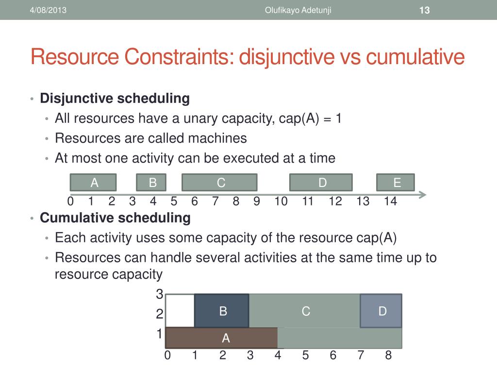
In the last lesson, we focused on machines in a job shop, which are a classic example of a disjunctive or unary resource. This means the resource has a capacity of one and can only process a single activity at a time. The noOverlap constraint is the perfect tool for this.

However, many real-world industrial systems involve cumulative resources, which have a capacity greater than one. Think of a team of 5 assembly workers, a fleet of 3 forklifts, or a communication network with a certain bandwidth. These resources can handle multiple activities simultaneously, as long as the total demand at any point in time does not exceed the resource's capacity.

The image below clearly illustrates this fundamental distinction.

2. The noOverlap Constraint for Unary Resources

As a brief review, the noOverlap constraint is our primary tool for modeling disjunctive resources.

noOverlap([op1, op2, ..., opN])

This single line of code enforces that for a given set of interval variables (representing operations on the same machine), no two intervals that are present in the final schedule can overlap. It elegantly replaces the complex "big-M" disjunctions we would need in a Mixed-Integer Linear Programming (MILP) model.

To see this constraint in action, you can refer back to Model 1 in the paper "Interval-Based Language for Modeling Scheduling Problems", which we looked at in the last lesson. Line 19 uses noOverlap to model the machines in a flow shop.

3. Modeling Cumulative Resources

Now, let's move to the main topic of today's lesson: modeling resources with a capacity greater than one. This is where the true power and expressiveness of CP for scheduling begin to shine.

Instead of a simple "no overlap" rule, we need to track the total resource consumption over time and ensure it never exceeds a capacity limit. CP solvers provide a powerful abstraction for this: the cumul function expression.

Cumul Function Expressions

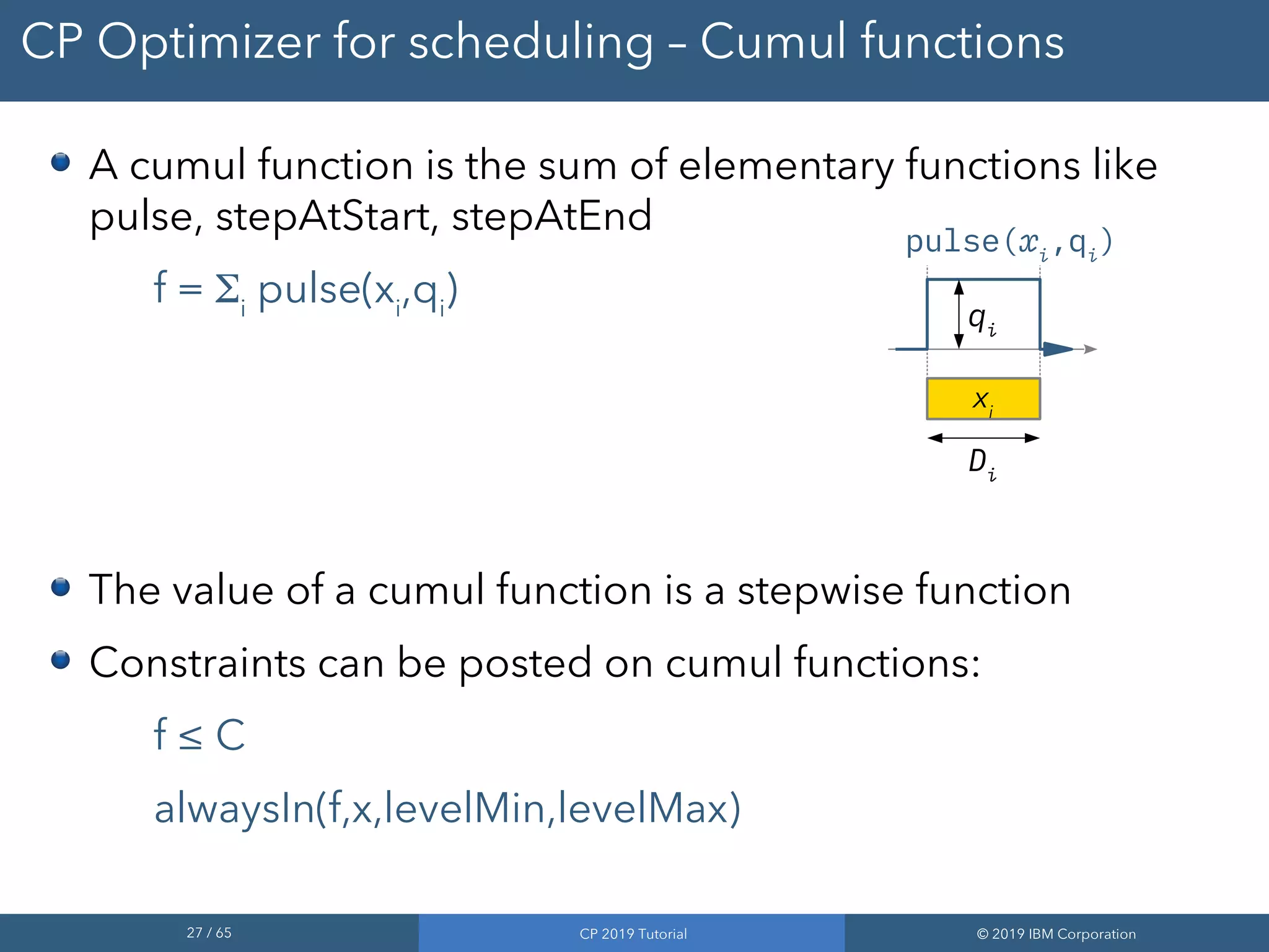
A cumul function represents the total usage of a resource over time. It is built by summing up the contributions of individual activities. The most common contribution is a pulse.

• A pulse function, pulse(interval, demand), states that during the time an interval is active, it consumes demand units of a resource.
• A cumul function is then the sum of these pulses: f = sum(pulse(op_i, demand_i)).
• The final constraint is simply to state that this function f must always be less than or equal to the resource's total capacity C: f <= C.

The image below, from a CP Optimizer tutorial, visualizes this concept perfectly.

For a formal and detailed explanation of how these functions work, please read the following section from the paper by Laborie et al.

Example: Modeling a Hybrid Flow Shop Stage

The cumul function is the ideal tool for modeling a stage in a Hybrid Flow Shop (HFS). An HFS is like a regular flow shop, but at least one stage has multiple parallel machines.

Let's say a stage has a pool of k identical machines. A set of operations op_1, op_2, ..., op_n must be processed at this stage. Each operation requires one machine.

We can model this pool of k machines as a single cumulative resource with capacity k. Each operation op_i requires 1 unit of this capacity. The model becomes remarkably simple:

1. Variables: Define an interval variable op_i for each operation.
2. Constraint: Create a single cumulative constraint:
   ${\sum }_{i=1}^n\text{pulse}({\text{op}}_i,1)\le k$

This constraint ensures that at any point in time, no more than k operations are running in parallel, which perfectly models the k parallel machines. This is far more direct and efficient than trying to model individual machine assignments.

Let's look at a complete model that uses this exact idea.

4. State Functions: Modeling Resources with Changing States

To round out our tour of global constraints for resources, let's look at one more type: State Functions. These are used to model a resource that doesn't have a numerical capacity, but rather exists in one of several discrete "states" over time.

Examples from an industrial context include:

• A machine that can be fitted with different tools (the state is the current tool).
• A chemical reactor that can be set to different temperatures or pressures (the state is the current setting).
• A paint booth that can be configured for different colors (the state is the current color).

A key aspect of state functions is modeling the transition time between states (e.g., the time it takes to change a tool or heat an oven). This makes them the perfect tool for modeling sequence-dependent setup times, a critical topic for your thesis that we will cover in detail in Module 7.

The main constraints on a state function f and an interval a are:

• alwaysEqual(f, a, v): Requires that during interval a, the resource state must be v.
• alwaysConstant(f, a): Requires that the state remains constant during interval a, whatever that state may be.

Conclusion

In this lesson, we significantly expanded our ability to model real-world resources using the specialized global constraints offered by Constraint Programming.

Key Takeaways:

• Scheduling problems involve two main types of resources: disjunctive (unary capacity) and cumulative (capacity > 1).
• The noOverlap constraint is used for disjunctive resources.
• Cumul function expressions, built from pulse functions, are the standard way to model cumulative resources. The constraint sum(pulse) <= C is a powerful and flexible tool, especially for modeling parallel machines in environments like Hybrid Flow Shops.
• State functions are used to model resources whose condition is described by a state rather than a numerical capacity. They are fundamental for modeling sequence-dependent setup times.

Preview of the Next Lesson:

We have now learned what the key building blocks of a CP scheduling model are: interval variables, temporal constraints, and powerful global constraints like noOverlap and Cumulative. You might be wondering how the solver can possibly handle these high-level concepts efficiently.

In our next lesson, we will look under the hood to answer that question. We will explore the core solving mechanism in CP: constraint propagation and domain reduction. You will learn how each constraint actively participates in the search by removing impossible values from the domains of variables, rapidly pruning the search space and enabling the efficient solution of complex scheduling problems.