Job Shop Scheduling with CP

1. Understanding the Job Shop Problem

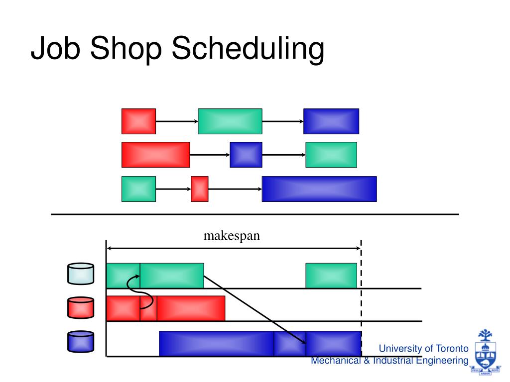
First, let's clearly define the problem we are solving. The Job Shop Scheduling Problem (JSSP) consists of:

• A set of jobs that need to be processed.
• A set of machines.
• Each job consists of a sequence of operations (or tasks), each of which must be processed on a specific machine for a given duration.

The problem is governed by two main types of constraints:

1. Precedence Constraints: The operations within a single job must be performed in a specified order.
2. Disjunctive (or Capacity) Constraints: Each machine can only process one operation at a time. Two operations assigned to the same machine cannot overlap.

The most common objective is to find a schedule that minimizes the makespan ($C_{max}$), which is the time when all jobs are completed.

This image provides an excellent visual summary of the problem.

2. The CP Modeling Approach for Scheduling

Before diving into the code, let's think about how we can represent the JSSP using the CP concepts we've learned. How do we translate jobs, machines, and constraints into the language of a CP solver?

The modern CP approach for scheduling uses specialized variables and constraints designed for this purpose. The following video by Prof. Pascal Van Hentenryck, a leading expert in the field, gives a concise overview of how a JSSP is modeled at a high level.

As the video explains, the core building blocks of our model will be:

• Interval Variables: Each operation will be modeled as an interval variable. This is a powerful abstraction that represents an activity with a start time, an end time, and a duration. The solver's goal is to find the start and end times for all these intervals.
• Precedence Constraints: For a job where operation A must precede operation B, we'll add a constraint: end_of(A) <= start_of(B).
• No-Overlap Constraint: For each machine, we will collect all the interval variables corresponding to operations that run on it and apply a single noOverlap global constraint. This constraint ensures that none of those intervals overlap in time and encapsulates the sophisticated propagation algorithms we discussed in the last lesson.

For a more formal and detailed description of these modeling concepts, the following paper by one of the designers of IBM's CP Optimizer is an excellent reference.

3. Implementing a JSSP Model with Google OR-Tools

Now, let's walk through the implementation of a JSSP model step-by-step. We will use Google's OR-Tools, a popular open-source library that includes a powerful CP-SAT solver. The following tutorial from the OR-Tools documentation will be our primary guide. We'll focus on the Python implementation, as it's very readable and widely used in research.

Let's begin.

Step 1: Define the Problem Data

First, we need a structured way to represent the problem instance. The standard format is a list of jobs, where each job is a list of tasks. Each task is a tuple containing the (machine_id, processing_time).

Referencing the "Define the data" section of the OR-Tools guide (LINK, section 3), we can see the data for a simple 3-job, 3-machine problem:

jobs_data = [
    # task = (machine_id, processing_time)
    [(0, 3), (1, 2), (2, 2)],  # Job 0
    [(0, 2), (2, 1), (1, 4)],  # Job 1
    [(1, 4), (2, 3)],         # Job 2
]

For example, the first task of Job 0 runs on machine 0 for 3 time units.

Step 2: Create the Model and Variables

Next, we create the model and declare our decision variables. For each task in our jobs_data, we need to create an interval variable. In OR-Tools, an interval variable is defined by a start integer variable, a fixed duration (processing time), and an end integer variable.

The code in the "Define the variables" section of the guide (LINK, section 4) does exactly this. It iterates through each job and task, creating:

• A start_var with a domain from 0 to a large upper bound (horizon).
• An end_var.
• An interval_var that links the start, duration, and end with the constraint start_var + duration = end_var.

It also usefully stores all interval variables belonging to the same machine in a dictionary machine_to_intervals. This will be crucial for the next step.

Step 3: Define the Constraints

This is where we enforce the rules of the job shop.

1. No-Overlap Constraints:
For each machine, we simply apply the AddNoOverlap global constraint to the list of intervals that run on it. As shown in the "Define the constraints" section (LINK, section 5), this is remarkably concise:

# Create and add disjunctive constraints.
for machine in all_machines:
    model.add_no_overlap(machine_to_intervals[machine])

This single line per machine invokes the powerful filtering algorithms that prevent any two operations on that machine from overlapping.

2. Precedence Constraints:
We also need to enforce the order of operations within each job. We iterate through each job and for every pair of consecutive tasks, we add a constraint stating that the first task must end before the second one begins.

# Precedences inside a job.
for job_id, job in enumerate(jobs_data):
    for task_id in range(len(job) - 1):
        model.add(all_tasks[job_id, task_id + 1].start >= all_tasks[job_id, task_id].end)

Step 4: Define the Objective

Our goal is to minimize the makespan. The makespan is defined as the maximum of the completion times of all jobs. The completion time of a job is simply the end time of its last operation.

As seen in the "Define the objective" section (LINK, section 6), we create a new integer variable to represent the makespan (obj_var) and constrain it to be equal to the maximum of the end times of the final tasks of all jobs.

# Makespan objective.
obj_var = model.new_int_var(0, horizon, "makespan")
model.add_max_equality(
    obj_var,
    [all_tasks[job_id, len(job) - 1].end for job_id, job in enumerate(jobs_data)],
)
model.minimize(obj_var)

The AddMaxEquality is another specialized constraint that efficiently propagates information between the makespan variable and the individual job completion times.

Step 5: Solve and Display the Results

The final steps are to create a solver instance, solve the model, and print the results. The code in the sections "Invoke the solver" and "Display the results" (LINK, sections 7 and 8) shows how to do this. After a successful solve, you can query the optimal value of any variable using solver.value(variable_name).

Conclusion

In this lesson, you have learned how to construct a complete Constraint Programming model for the classic Job Shop Scheduling Problem. We've seen how high-level abstractions provided by CP solvers allow us to model the problem in a way that is both declarative and powerful.

Key Takeaways:

• The JSSP is defined by precedence constraints within jobs and disjunctive constraints on machines.
• In CP, we model operations as interval variables.
• Precedence is modeled with simple end <= start linear constraints.
• Machine capacity is modeled efficiently using the NoOverlap global constraint, which handles all the disjunctive logic and propagation for a resource.
• The makespan objective is modeled by finding the maximum end time of the last operation of all jobs, often using a dedicated MaxEquality constraint.
• The overall modeling process is a clear, step-by-step translation of the problem's rules into the solver's language.

Preview of the Next Lesson:

We now have a solid model for the standard job shop. But your thesis focuses on the Flexible Job Shop Problem (FJSP), where an operation has a choice of machines it can be processed on. In our next lesson, we will extend our CP model to solve the FJSP by incorporating alternative interval variables. You will see how CP's modeling capabilities make this extension surprisingly elegant.