Hello! Welcome to the first lesson in our module on Constraint Programming.
In the previous module, we explored several metaheuristics—like Genetic Algorithms, Simulated Annealing, and Tabu Search—which are designed to find high-quality solutions to complex optimization problems. These methods work by intelligently exploring a vast search space, but they don't guarantee finding the absolute best solution.
Today, we shift paradigms from heuristics to exact methods. We will begin our study of Constraint Programming (CP), a powerful framework for modeling and solving combinatorial problems. Our goal for this lesson is to define constraint satisfaction and constraint optimization problems. Understanding this distinction is the first and most crucial step toward mastering CP, which you'll find is a very different yet powerful tool for your thesis work on Flexible Job Shop Problems.
1. What is a Constraint Satisfaction Problem (CSP)?
In our previous lessons on search and metaheuristics, we often thought about problems in terms of states, actions, and finding a path or sequence of moves to a goal. A state was often a "black box" that we could only query with a successor function or a goal test.
Constraint Programming approaches problems differently. It's an example of an identification problem, where the goal is not the path, but the final assignment of values to variables that meets a set of rules. CP gives us a structured, declarative language to describe these rules.
A CSP is formally defined by three components:
- Variables: A set of decision variables, .
- Domains: For each variable , there is a domain of possible values it can take.
- Constraints: A set of constraints that specify the allowed combinations of values for subsets of the variables.
A solution to a CSP is a complete assignment of a value from its domain to every variable such that all constraints are satisfied. The task is to find such a solution or determine that none exists.
To get a more intuitive feel for this, let's watch a video that introduces CSPs using the classic map-coloring problem.
COMPSCI 188 - 2018-09-04 - Constraint Satisfaction Problems (CSPs) Part 1/2
This video from Berkeley's AI course provides an excellent introduction to CSPs. It contrasts them with the standard search problems we've seen before and clearly breaks down the components using the map-coloring example.
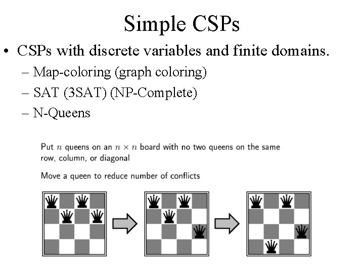
Please watch from 08:34 to 17:59. Focus on how a problem is broken down into variables, domains, and constraints. Notice the N-Queens example as well; it's another classic CSP.
As the video explained, problems like map coloring and N-Queens are canonical examples of CSPs.
Given your background in industrial engineering, let's look at how a simple scheduling problem can be modeled as a CSP. The way you define your variables and constraints is a critical modeling choice that can significantly impact how easy the problem is to solve.
Factor Graphs 1 - Constraint Satisfaction Problems | Stanford CS221: AI (Autumn 2019)
This video from a Stanford AI course demonstrates how to model an event scheduling problem as a CSP. Pay close attention to the discussion of two different formulations—one where events are variables and another where time slots are variables. This highlights the flexibility and power of CP modeling.
Please watch from 01:10:38 to 01:18:34. The key takeaway is understanding that the same problem can be modeled in different ways within the CSP framework, and these choices have practical consequences for the solver.
2. From Satisfaction to Optimization (COP)
So far, we've only talked about satisfying constraints. The goal in a CSP is to find any solution that works. This is known as a decision problem.
However, in most real-world scheduling scenarios, including your thesis on FJSP, you don't just want any feasible schedule; you want the best one according to some performance metric (like minimizing makespan). This is a Constraint Optimization Problem (COP).
A COP is simply a CSP plus an objective function.
To understand the relationship between them, we can use a more general concept called a Factor Graph.
Factor Graphs 1 - Constraint Satisfaction Problems | Stanford CS221: AI (Autumn 2019)
Let's return to the Stanford video, which introduces factor graphs. This provides a unified view of both satisfaction and optimization problems.
Watch from 13:34 to 21:09 and then from 30:08 to 34:31. The first segment defines factor graphs, where each 'factor' assigns a score or weight to a partial assignment. The second segment explains that a CSP is a special case where factors are binary (0 or 1), representing hard constraints. If the total weight (product of factors) is 1, the assignment is valid; if 0, it's invalid.
As the video explains, a CSP is a factor graph where all factors are hard constraints that return either 1 (satisfied) or 0 (violated). The goal is to find an assignment with a total weight of 1.
A COP can be seen as a factor graph where factors can return non-negative weights representing costs or preferences. The goal becomes finding the assignment that maximizes (or minimizes) the total weight.
In practice, COPs are often solved by iteratively solving a sequence of CSPs. This is a crucial technique in the CP world.
Constraint Programming for Scheduling
The following document, 'Constraint Programming for Scheduling', clearly explains how the CSP algorithm is adapted to solve optimization problems.
Please read section 47.3.4 Adapting the CSP Algorithm to Constrained Optimization Problems. This short section describes the standard 'branch-and-bound' like process for solving a COP.
The process is as follows for a minimization problem:
- Find a feasible solution to the initial CSP. Let its objective value be .
- Add a new constraint to the model:
ObjectiveValue <. - Solve this new, more restrictive CSP. If a solution is found, update with the new, better objective value and repeat step 2.
- If the CSP becomes unsatisfiable, it means no better solution exists. The last solution found is the proven optimum.
Test your understanding!
Consider a simple scheduling problem with two jobs, J1 and J2, on a single machine.
- J1 has processing time .
- J2 has processing time .
The machine can only process one job at a time.
How would you formulate this as a Constraint Satisfaction Problem (CSP) to find any schedule that finishes by time 10? Define the variables, their domains, and the constraints.
Show answer
Here is one possible formulation:
-
Variables:
- : Start time of Job 1.
- : Start time of Job 2.
-
Domains:
- Since the schedule must start at or after time 0 and finish by time 10:
- Domain of : .
- Domain of : .
-
Constraints:
- Finish by deadline:
- (This is already encoded in the domain).
- (This is also encoded in the domain).
- No overlap (disjunctive constraint): The time intervals and cannot overlap. This is expressed as:
- OR .
- Finish by deadline:
Any pair of values from the domains that satisfies the "No overlap" constraint is a solution. For example, is a valid solution.
Now, how would you change this into a Constraint Optimization Problem (COP) to minimize the makespan ()? The makespan is the time the last job finishes.
Show answer
To turn it into a COP, we add an objective function and a variable to represent it.
-
Variables, Domains, Constraints: Same as above, but we can relax the strict domains based on the time 10 deadline, as the optimizer will handle it.
- Domains: .
-
Additional Variable:
- : The makespan of the schedule.
-
Additional Constraints:
These two constraints define the makespan as the completion time of the last job to finish.
-
Objective Function:
- Minimize .
The solver would then use the iterative process described earlier to find the assignment for and that minimizes while respecting the disjunctive constraint. The optimal solution is (or vice versa), for a makespan of 8.
Conclusion
This lesson introduced the fundamental concepts of Constraint Programming. We have laid the groundwork for a new way of thinking about and solving the complex scheduling problems central to your research.
Key Takeaways:
- A Constraint Satisfaction Problem (CSP) is defined by a set of variables, their domains, and constraints on those variables. The goal is to find a single feasible assignment.
- A Constraint Optimization Problem (COP) is a CSP with an added objective function to be minimized or maximized.
- Modeling a problem in CP involves making key decisions about what the variables and constraints will be, which can significantly affect solver performance.
- COPs are typically solved by iteratively finding a feasible solution and then adding a new constraint that requires the next solution to be strictly better, until no more solutions can befound.
Preview of the Next Lesson:
Now that we have the abstract definitions, our next step is to apply them to a realistic scheduling problem. In the next lesson, we will learn how to model a job shop scheduling problem using interval variables and temporal constraints. We'll see how CP allows for rich variable types beyond simple integers and how specialized "global constraints" can elegantly capture complex scheduling rules like resource non-overlap. This will be our first concrete step in building a CP model for problems like the FJSP.