CP vs. MILP for Scheduling: Strengths & Weaknesses

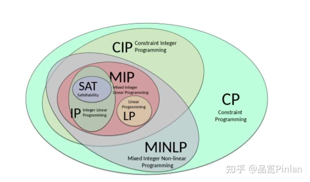
1. Two Paradigms: Core Differences in Modeling and Solving

At their heart, MILP and CP represent two different ways of thinking about and solving the same problem. The differences begin with how you even describe the problem to the computer.

Modeling Philosophy

• Mixed-Integer Linear Programming (MILP): A MILP model is purely declarative and mathematical. You define a set of decision variables (which can be real or integer), a linear objective function to minimize or maximize, and a set of linear inequalities or equalities that the variables must satisfy. Any non-linear or logical relationship must be "linearized." For scheduling, this often involves using the "big-M" formulation to represent disjunctive constraints (e.g., "operation A is before B" OR "B is before A").

• Constraint Programming (CP): CP offers a much richer and more expressive modeling language. While still declarative, it allows you to use "global constraints," which are powerful modeling objects that encapsulate complex combinatorial substructures. Instead of using a "big-M" formulation to prevent two operations from overlapping, you can simply state NoOverlap(operations_on_machine_k). The solver knows what a NoOverlap constraint means and has specialized algorithms to reason about it.

Solution Approach

This difference in modeling leads to a fundamental difference in how solvers search for a solution. Both typically use a branching search (building a search tree), but what they do at each node of the tree is worlds apart.

• MILP Solvers (Branch-and-Cut):

  1. Relaxation: At each node, the solver relaxes the integrality constraint (e.g., a variable that must be 0 or 1 is allowed to be 0.5). This creates a Linear Program (LP), which can be solved very efficiently.
  2. Bounding: The solution to the LP provides a bound on the best possible objective value in that part of the search tree. If this bound is worse than a known integer solution, the entire branch of the tree can be pruned.
  3. Branching: If the LP solution has fractional values for integer variables, the solver branches by creating two new subproblems (e.g., one where x=0 and one where x=1).

• CP Solvers (Branch-and-Propagate):

  1. Propagation: At each node, the solver uses the constraints to reduce the domains (the set of possible values) of the decision variables. For example, if operation A (duration 5) must end by time 10, the EndBeforeStart constraint will propagate this information to deduce that operation A must start no later than time 5, reducing its domain. This is also called domain filtering or inference.
  2. Pruning: If any variable's domain becomes empty, the solver knows the current path is infeasible and backtracks.
  3. Branching: If propagation finishes and variables still have multiple values in their domains, the solver branches by splitting a domain (e.g., trying a specific start time for an operation).

To get a concise overview of these differences, please read the following material from a classic tutorial on Constraint Programming by John Hooker.

2. A Tale of Two Toolkits: Strengths and Weaknesses

As the reading from Hooker's tutorial highlights, neither method is universally superior. Their strengths are complementary.

Strengths of Constraint Programming (CP)

• Expressive Modeling: Global constraints for scheduling (NoOverlap, Cumulative), sequencing (AllDifferent), and logic (Alternative) make models easier to write, read, and maintain.
• Strong on Combinatorics: Excels at problems with heavy combinatorial logic, sequencing, and resource allocation—the very essence of scheduling.
• Effective Propagation: For problems where LP relaxations are weak (like scheduling), constraint propagation can prune the search space much more effectively. Adding more constraints can often speed up the search by enabling more propagation.

Strengths of Mixed-Integer Linear Programming (MILP)

• Powerful Relaxations: For problems that have a "good" linear structure (e.g., network flow, many assignment problems), the LP relaxation provides very tight bounds, allowing the solver to prune huge sections of the search tree.
• Mature Solvers: MILP solvers are a highly mature technology, incredibly optimized for solving LPs and employing sophisticated techniques like automatic cut generation to strengthen relaxations.
• Dominance on Cost-Based Objectives: When the objective function is a linear combination of variables and the problem has many "knapsack-like" constraints, MILP is often unbeatable.

For scheduling, the key weakness of MILP is its reliance on weak "big-M" formulations for disjunctions. The key strength of CP is its ability to reason about these disjunctions directly and powerfully through global constraints.

3. Case Study: FJSP Performance in Practice

Theory is one thing, but performance on real problems is what matters. The paper by Kasapidis et al. provides a perfect head-to-head comparison of MILP and CP on the Flexible Job Shop Problem, including the more general variant with arbitrary precedence graphs that is relevant to your thesis work.

First, let's look at how they formulated the problem using each paradigm. You are already familiar with the CP approach from our last lesson. Now, let's examine the MILP formulation.

Now for the crucial question: which one performs better? The paper provides extensive computational results that paint a very clear picture.

The empirical evidence from this research is overwhelming and consistent with scheduling theory:

• CP is significantly more effective than MILP for the FJSP. Across all benchmark sets, the CP model finds better solutions (lower makespans) and proves optimality much more often than the MILP model within the same time limit.
• As the problem size and complexity grow, the performance gap widens. The authors note that for many instances, the "MIP failed even to produce feasible upper bounds," whereas the CP model found high-quality solutions.
• This demonstrates that for complex scheduling problems like FJSP, the powerful, specialized inference of CP's global constraints (NoOverlap, Alternative) far outweighs the general-purpose bounding mechanism of MILP's LP relaxations, which are crippled by the weak "big-M" formulations.

Conclusion

In this lesson, we have conducted a detailed comparison of the two leading paradigms for exact optimization: CP and MILP. You now have a solid understanding of not just what they are, but why they perform differently on scheduling problems.

Key Takeaways:

• Different Philosophies: MILP uses a purely mathematical formulation with linear constraints, while CP uses a richer language with global constraints that capture combinatorial substructures.
• Different Solution Engines: MILP solves LP relaxations for bounds (Branch-and-Cut), while CP uses constraint propagation to filter variable domains (Branch-and-Propagate).
• Scheduling Favors CP: For problems like JSSP and FJSP, the weak LP relaxations of standard MILP models make them struggle. CP's ability to reason intelligently about scheduling-specific constraints gives it a decisive advantage.
• Justification for Your Thesis: The evidence strongly suggests that for complex FJSP variants, CP is the more powerful and appropriate exact method. You can now confidently cite both theoretical reasons (expressive modeling, strong propagation) and empirical evidence (e.g., Kasapidis et al.) to support this choice.

Preview of the Next Lesson:

While we've positioned CP and MILP as competing approaches, their strengths are also complementary. This has led to a fascinating and highly effective research area: hybrid optimization methods. In our next module, we will explore how to combine the strengths of different methods. We'll begin by looking at the motivation for combining metaheuristics (like the Evolutionary Algorithm in the paper we just read) with exact methods like CP, creating powerful solvers that can tackle even larger and more complex industrial problems.