Hello! Welcome to your next lesson in our journey through Flow Shop Scheduling.
In our last session, we formally defined the permutation flow shop problem (PFSP) and its underlying assumptions. We established that for a given set of jobs, our main task is to find the best processing sequence, or permutation, that optimizes an objective, typically the makespan ().
Today, we'll build directly on that foundation by addressing the learning outcome: Represent flow shop schedules using Gantt charts. This lesson is all about visualization. We will move from the abstract concept of a job sequence (e.g., J2-J4-J1-...) to a concrete, visual representation of how that sequence unfolds over time on the machines. This skill is indispensable for analyzing schedule quality, identifying bottlenecks, and communicating results—all critical aspects of the research you'll be doing for your thesis.
1. What is a Gantt Chart?
A Gantt chart is the most common and intuitive tool for visualizing a schedule. In the context of shop scheduling, it plots machine activity against a timeline. Given your background in industrial engineering, you have likely encountered Gantt charts in project management; their application here is very similar.
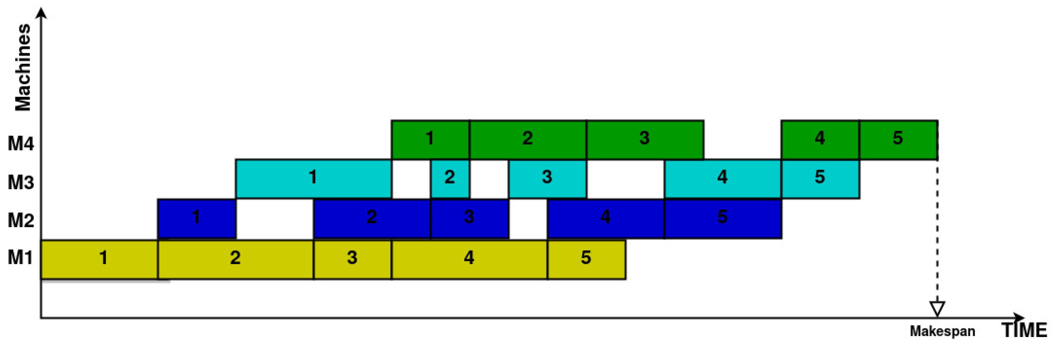
A schedule's Gantt chart typically has:
- A horizontal axis representing elapsed time.
- A vertical axis listing the machines in the shop.
- Bars or blocks on the chart, where each bar represents a specific operation (job on machine ) and its length corresponds to the processing time.
The following document provides a concise introduction.
The lecture notes on 'Job Shop Scheduling' offer a clear and straightforward definition of the Gantt chart and its purpose in scheduling.
Please read the section titled 'Gantt Chart' (it's on the first page). Focus on its definition as a 'graphical display technique' and what it helps to evaluate (makespan, idle time, etc.).
As the reading states, a Gantt chart isn't an optimization tool itself, but a way to display and evaluate the results of a scheduling decision. By looking at a Gantt chart, we can immediately see the flow of jobs, periods where machines are idle, and when the very last operation finishes, which defines the makespan.
Below is a typical Gantt chart for a permutation flow shop problem with 5 jobs and 4 machines.
2. How to Construct a Gantt Chart
Now, let's move to the main task: how do we get from a problem definition (jobs, machines, processing times) and a given sequence to the chart itself? The process follows a set of logical rules derived directly from the PFSP assumptions we learned in the last lesson.
The key is to determine the start time for each operation. An operation (job on machine ) can only begin when two conditions are met:
- Job Readiness: The job itself must be ready. This means it must have completed its processing on the previous machine, .
- Machine Availability: The machine must be free. This means it must have finished processing the previous job in the sequence.
Therefore, the start time of an operation is the maximum of these two events.
The following video provides an excellent walkthrough of this logic. It verbally describes the step-by-step placement of each job's operations on a Gantt chart.
The scheduling problem (7/7). Computation of makespan in a permutation flow shop
The video 'The scheduling problem (7/7). Computation of makespan...' by Luis R. Izquierdo explains the logic for building a schedule for a given sequence.
Please watch from 00:39 to 08:16. The video will first introduce an example problem (00:39-02:26). Then, pay close attention as the narrator explains how the Gantt chart is constructed for the sequence 4-2-5-1-3 (02:40-06:11). Finally, the video formalizes the 'maximum' rule we just discussed (06:11-08:16).
Let's solidify this with our own small example.
Consider a 3-job, 2-machine problem with the following processing times ():
| Job | Machine 1 | Machine 2 |
|---|---|---|
| J1 | 4 | 5 |
| J2 | 2 | 3 |
| J3 | 6 | 2 |
Let's construct the Gantt chart for the sequence J1-J2-J3.
Step 1: Schedule Job 1 (first in sequence)
- J1 on M1: Starts at . Finishes at .
- J1 on M2: Ready at . M2 is free. Starts at . Finishes at .
Step 2: Schedule Job 2 (second in sequence)
- J2 on M1: Can start when M1 is free. M1 finishes J1 at . Starts at . Finishes at .
- J2 on M2: Ready at (finished on M1). M2 is free at (finished J1). The start time is . Starts at . Finishes at . Notice the 3 units of idle time for J2 between M1 and M2, waiting for M2 to become free.
Step 3: Schedule Job 3 (third in sequence)
- J3 on M1: Can start when M1 is free. M1 finishes J2 at . Starts at . Finishes at .
- J3 on M2: Ready at (finished on M1). M2 is free at (finished J2). The start time is . Starts at . Finishes at .
The makespan is the completion time of the last operation (J3 on M2), which is 14.
Test your understanding!
Using the same 3-job, 2-machine problem data from above, construct the Gantt chart for the sequence J2-J1-J3. What is the new makespan? Does this sequence perform better or worse?
Show answer
Let's build the schedule for the sequence J2-J1-J3:
Step 1: Schedule Job 2
- J2 on M1: Starts at , finishes at .
- J2 on M2: Starts at , finishes at .
Step 2: Schedule Job 1
- J1 on M1: Starts when M1 is free (after J2), at . Finishes at .
- J1 on M2: Ready at . M2 is free at . Start time is . Finishes at . Note the 1 unit of idle time on M2 from t=5 to t=6.
Step 3: Schedule Job 3
- J3 on M1: Starts when M1 is free (after J1), at . Finishes at .
- J3 on M2: Ready at . M2 is free at . Start time is . Finishes at .
The makespan for the sequence J2-J1-J3 is 14. In this case, both sequences resulted in the same makespan.
3. Comparing Schedules with Gantt Charts
The primary goal of solving a PFSP is to find the sequence with the best makespan. Gantt charts are the perfect tool for comparing different candidate sequences. By drawing the chart for each, you can visually confirm which one finishes earliest.
The following resource provides several examples of Gantt charts for the same problem but with different sequences, clearly showing how the makespan changes.
Permutation Flow Shop via Simulated Annealing and NEH
This thesis chapter, 'Permutation Flow Shop via Simulated Annealing and NEH', visually demonstrates the impact of job sequencing on makespan.
Please go to Section 2.4.1, 'Example' (page 11). Look at the problem data in Table 2.2. Then, examine Figures 2.2, 2.3, 2.4, and 2.5 on page 12. Each figure is a Gantt chart for a different job sequence. Notice how the visual structure and the final makespan change dramatically with the sequence.
As you can see from the figures, the sequence has a profound impact.
- The sequence in Figure 2.4 results in a makespan of 78. You can see significant gaps (idle time) on the later machines.
- The sequence in Figure 2.5, however, creates a much more compact schedule, with less idle time and a makespan of only 56.
This visual feedback is invaluable. It helps build intuition about what makes a "good" schedule—typically, one that avoids starving later machines for work and minimizes overall idle time.
Conclusion
In this lesson, we have translated the abstract definition of a permutation flow shop schedule into a tangible, graphical representation. This is a foundational skill for the rest of the course and for your future research.
Key Takeaways:
- Gantt charts are the standard method for visualizing schedules, showing machine activity over time.
- The construction of a Gantt chart for a PFSP is governed by a simple but powerful rule: an operation can only start when both the job is ready (finished on the previous machine) and the machine is available (finished the previous job).
- Gantt charts allow for the direct identification of the makespan, as well as other important features like machine idle time and job waiting time.
- By comparing Gantt charts for different sequences, we can visually and quantitatively assess which schedule is better.
Preview of the Next Lesson:
While drawing a Gantt chart is excellent for understanding, it can be slow and cumbersome. For an algorithm to evaluate thousands of sequences, it needs a faster method. In the next lesson, we will formalize the construction logic you learned today into a set of recursive equations. This will allow us to calculate the makespan for any given sequence purely mathematically, without needing to draw a chart every time.