Calculating Age-Specific Mortality Rates

Introduction

In our previous lesson, we tackled the practical challenge of estimating population counts from incomplete data, such as periodic censuses. This allowed us to calculate the 'exposed to risk'—a crucial denominator for any mortality investigation. Now that we know how to quantify the population exposed to the risk of death, we can move to the next logical step: calculating the mortality rate itself.

This lesson introduces the fundamental tool for this task: the life table. We will explore its structure and the relationships between its core components. Our main goal is to understand and apply the actuarial estimate, which is the standard method for calculating age-specific mortality rates ( $q_{x}$ ) from life table data. This will formalize the connection between the raw data (lives and deaths) and the probability of death, a cornerstone of actuarial work.

The Life Table: A Portrait of Mortality

At its heart, a life table is a concise, tabular summary of the mortality experience of a population. It tracks a hypothetical cohort of people from a starting age (often birth) and shows how many survive from one age to the next.

For your reference, here is an example of a complete life table, showing the typical columns an actuary would work with.

This is an example of an abridged life table for Australian males, illustrating the key metrics used to track mortality and survival across different ages.

The core of any life table revolves around a few key functions. Let's define them formally.

Chapter 3 - Life Tables

This document provides a clear, mathematical introduction to the fundamental components of a life table.

Please read the first few pages of the chapter, focusing on the definitions of the basic life table quantities. Start at the beginning of Section 3.2 and read up to the introduction of the quantity L_x. Pay close attention to the definitions of: Radix and Survivors (l_x): The number of individuals alive at the exact integer age x. The starting number, l_0, is called the radix. Mortality Probability (q_x): The probability that an individual aged exactly x will die before reaching age x+1. Number of Deaths (d_x): The expected number of deaths between age x and age x+1.

As the reading highlights, these quantities are all interconnected. The entire table can typically be constructed if you know just one of the columns (e.g., all the $l_{x}$ values or all the $q_{x}$ values) and a starting radix. The fundamental relationships are:

Number of deaths: The number of people who die in the year of age $x$ is the difference between the number who were alive at the start of the year and the number alive at the end. $d_{x} = l_{x} - l_{x + 1}$
Survival probability: The probability of a person aged $x$ surviving to age $x + 1$ , denoted $p_{x}$ , is the ratio of survivors at $x + 1$ to those who started at age $x$ . $p_{x} = \frac{l _{x + 1}}{l _{x}}$
Mortality probability: Since death and survival are the only two outcomes, the probability of dying, $q_{x}$ , is complementary to the probability of surviving. $q_{x} = 1 - p_{x} = 1 - \frac{l _{x + 1}}{l _{x}} = \frac{l _{x} - l _{x + 1}}{l _{x}} = \frac{d _{x}}{l _{x}}$

The Actuarial Estimate

The relationship $q_{x} = d_{x} / l_{x}$ is the foundation of the actuarial estimate. Given your background in statistics, you can think of this as estimating a binomial probability. If you have $l_{x}$ independent "trials" (people alive at age $x$ ), and you observe $d_{x}$ "successes" (deaths), then the most natural estimator for the probability of success, $q_{x}$ , is the sample proportion:

q^_{x} = \frac{d _{x}}{l _{x}}

In actuarial science, we often generalize this. The denominator, $l_{x}$ , represents the initial exposed to risk—the count of lives at the beginning of the age interval who are at risk of dying during that interval. The estimator is more broadly written as:

q^_{x} = \frac{Number of deaths}{Initial exposed to risk} = \frac{d _{x}}{E _{x}}

In the simple context of a standard life table where no one enters or leaves the group mid-year (other than by death), the initial exposed to risk $E_{x}$ is simply $l_{x}$ . The term "actuarial estimator" is formally derived under an assumption about how deaths are distributed within the year (the Balducci assumption), which makes it robust when dealing with policies that lapse or are withdrawn mid-year. For our current purpose of applying it to life table data, the simple formula $q^_{x} = d_{x} / l_{x}$ is sufficient and correct.

Application: Completing a Life Table and Valuing Annuities

Let's put these relationships into practice with an exam-style problem. This exercise will require you to work backwards and forwards through the life table relationships to find missing values and then use those values in a financial calculation.

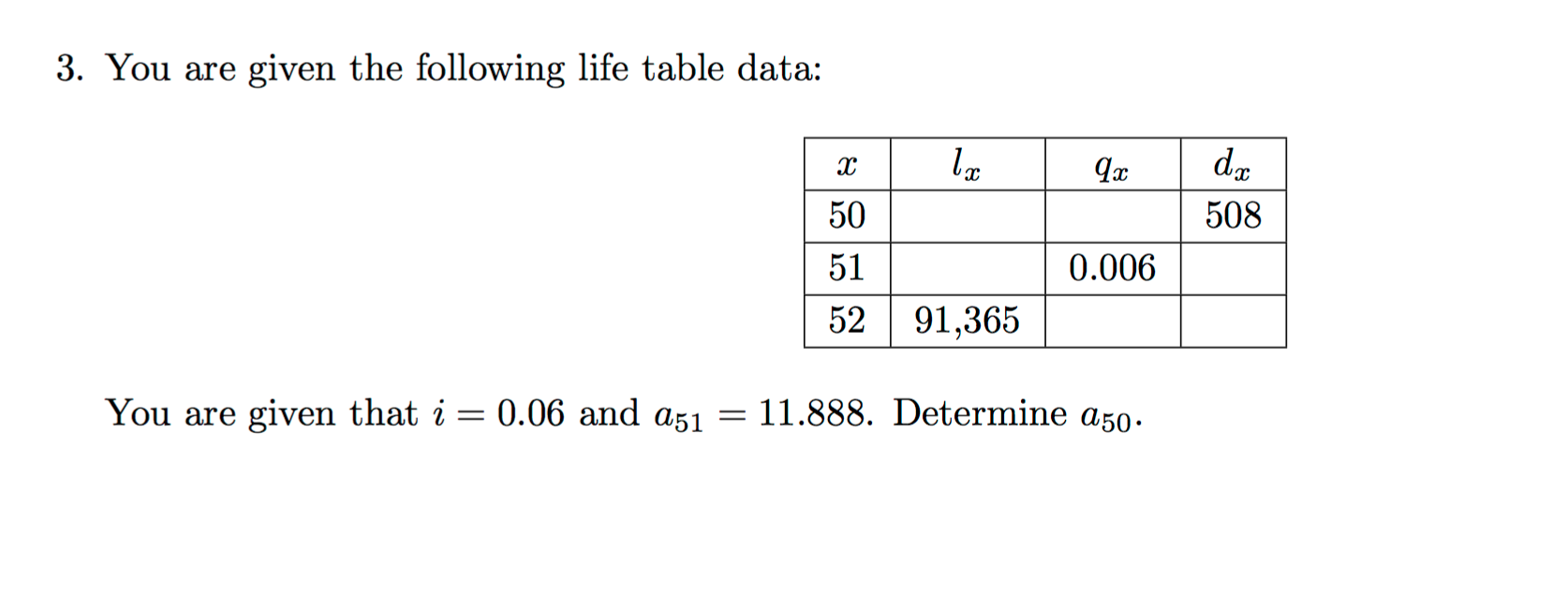
An example problem requiring the calculation of missing life table values and a life annuity value.

You are given a partially completed life table and are asked to determine $a_{50}$ , the present value of a whole life annuity-due for a person aged 50. The annuity pays 1 unit at the beginning of each year the person is alive. You're also given that the interest rate $i = 0.06$ and $a_{51} = 11.888$ .

Let's solve this step-by-step.

Step 1: Find $l_{51}$

We are given $q_{51} = 0.006$ and $l_{52} = 91, 365$ .
The survival probability at age 51 is $p_{51} = 1 - q_{51} = 1 - 0.006 = 0.994$ .
We know that $p_{51} = l_{52} / l_{51}$ . We can rearrange this to find $l_{51}$ :

l_{51} = \frac{l _{52}}{p _{51}} = \frac{91 , 365}{0.994} = 91, 916.5

Note that $l_{x}$ values don't have to be integers; they represent an expected number of survivors.

Step 2: Find $l_{50}$

We are given $d_{50} = 508$ .
The fundamental life table relationship is $l_{51} = l_{50} - d_{50}$ . Rearranging gives us $l_{50}$ :

l_{50} = l_{51} + d_{50} = 91, 916.5 + 508 = 92, 424.5

Step 3: Calculate $p_{50}$

Now that we have $l_{50}$ and $l_{51}$ , we can calculate the probability that a 50-year-old survives to age 51:

p_{50} = \frac{l _{51}}{l _{50}} = \frac{91 , 916.5}{92 , 424.5} \approx 0.994504

Alternatively, we could first calculate $q_{50} = d_{50} / l_{50} = 508/92, 424.5 \approx 0.005496$ , and then $p_{50} = 1 - q_{50}$ .

Step 4: Calculate $a_{50}$ using the recursive formula

The value of a life annuity-due, $a_{x}$ , can be expressed recursively. A person aged $x$ is certain to receive the first payment of 1 now. They will receive the subsequent payments (which are worth $a_{x + 1}$ at time 1) if they survive one year. Discounting this future value back to the present gives:

a_{x} = 1 + v \cdot p_{x} \cdot a_{x + 1}

where $v = 1/ (1 + i)$ is the discount factor.

We have all the pieces to find $a_{50}$ :

$v = 1/1.06$
$p_{50} \approx 0.994504$
$a_{51} = 11.888$

Plugging these in:

a_{50} = 1 + (\frac{1}{1.06}) \cdot (0.994504) \cdot (11.888)

a_{50} \approx 1 + (0.943396) \cdot (0.994504) \cdot (11.888) \approx 1 + 11.1534

a_{50} \approx 12.153

This calculation demonstrates the direct link between the fundamental mortality data in a life table and the financial calculations that underpin insurance and pension products.

Conclusion

In this lesson, we formalized the process of calculating mortality rates from observed data. You learned how to interpret the structure of a life table and use the relationships between its columns to solve for unknown values.

Key Takeaways:

A life table tracks a cohort of lives, showing survivors ( $l_{x}$ ), deaths ( $d_{x}$ ), and the associated probabilities of survival ( $p_{x}$ ) and mortality ( $q_{x}$ ).
These components are linked by simple but powerful formulas: $d_{x} = l_{x} - l_{x + 1}$ and $q_{x} = d_{x} / l_{x}$ .
The actuarial estimate for the mortality rate $q^_{x}$ is the ratio of observed deaths to the initial number of lives exposed to risk ( $E_{x}$ ), which in a simple life table is $l_{x}$ .
Mastering these relationships is essential for practical actuarial work, allowing you to move from raw data to pricing financial products like life annuities.

Preview of the Next Lesson

So far, we have estimated $q_{x}$ , the probability of death over a full year. However, mortality is a continuous process that unfolds day by day. In our next lesson, we will zoom in further to estimate the instantaneous rate of mortality, known as the force of mortality, $μ_{x}$ . We will explore how to estimate this continuous rate from discrete data using the powerful statistical method of maximum likelihood estimation.

Recommended resources