Ruin Probability: Lundberg's Inequality & Cramér-Lundberg Approximation

The Probability of Ultimate Ruin and Lundberg's Inequality

Let's start by formally defining the quantity we wish to estimate. The probability of ultimate ruin, denoted by $\psi (u)$, is the probability that the insurer's surplus process $U(t)=u+ct-S(t)$ ever drops below zero, given an initial surplus of $u$.

Calculating $\psi (u)$ exactly is often impossible for most realistic models. This is where the adjustment coefficient $R$ becomes indispensable. Lundberg's inequality provides a powerful, clean, and surprisingly simple upper bound for this probability.

As the video explained, Lundberg's inequality states:

This elegant result shows that the probability of ruin decreases exponentially as the initial surplus $u$ increases. The rate of this decay is governed by $R$. A larger adjustment coefficient (indicating a less risky portfolio) leads to a much faster reduction in ruin probability for each additional unit of capital.

The following resource provides a clear definition of the inequality and its underlying assumptions.

Application: Calculating the Ruin Bound

Let's apply this. Suppose an insurer's aggregate claims follow a compound Poisson process with claim frequency $\lambda =20$ per year. Individual claim sizes are exponentially distributed with a mean of $500. The insurer sets premiums with a safety loading of $\theta =25\%$.

1. Parameters:

   • $\lambda =20$
   • Claim size $X\sim \text{Exp}(\alpha )$, with mean $\mu =1/\alpha =500$, so $\alpha =0.002$.
   • Premium rate $c=(1+\theta )\lambda \mu =(1.25)(20)(500)=12,500$.

2. Calculate the Adjustment Coefficient (R):
   From our previous lesson, we know that for exponential claims, $R$ has a closed-form solution:

   $$R=\alpha -\frac{\lambda }{c}=0.002-\frac{20}{12,500}=0.002-0.0016=0.0004$$

3. Apply Lundberg's Inequality:
   What is the upper bound for the probability of ruin if the insurer starts with an initial surplus of $u=\$10,000$?

   $$\psi (10000)\le e^{-R\cdot u}=e^{-0.0004\cdot 10000}=e^{-4}\approx 0.0183$$

   So, there is at most a 1.83% chance that the insurer will ever be ruined.

The proof of Lundberg's inequality relies on a clever martingale argument, which is detailed in Section 2.1.2 of the UCSD Math Department notes (LINK). While you don't need to reproduce the proof for the exam, your background makes it an interesting read if you are curious.

From Bound to Approximation: The Cramér-Lundberg Result

Lundberg's inequality is an upper bound, which by its nature is conservative. For large values of initial surplus $u$, a more precise estimate is often needed. The Cramér-Lundberg approximation provides this by showing that as $u$ becomes large, the ruin probability behaves asymptotically like the exponential bound.

The approximation is given by:

where $C$ is a constant that is less than 1. This means the true ruin probability is slightly lower than the Lundberg bound, but follows the same exponential decay.

For the special case of exponentially distributed claims, the exact ruin probability is known, and it beautifully illustrates the Cramér-Lundberg form:

Here, the constant $C$ is simply $\frac{1}{1+\theta }$.

Let's revisit our previous example:

• $\theta =0.25$, $R=0.0004$, $u=10,000$.
• Lundberg's bound: $\psi (10000)\le e^{-4}\approx 0.0183$.
• Exact probability: $\psi (10000)=\frac{1}{1.25}{e}^{-4}=0.8\times 0.0183\approx 0.0147$.

As you can see, the exact probability (1.47%) is indeed less than the bound (1.83%), and the factor separating them is $C=0.8$.

For general claim distributions, an exact formula for $\psi (u)$ is unavailable, but the constant $C$ in the Cramér-Lundberg approximation can be calculated.

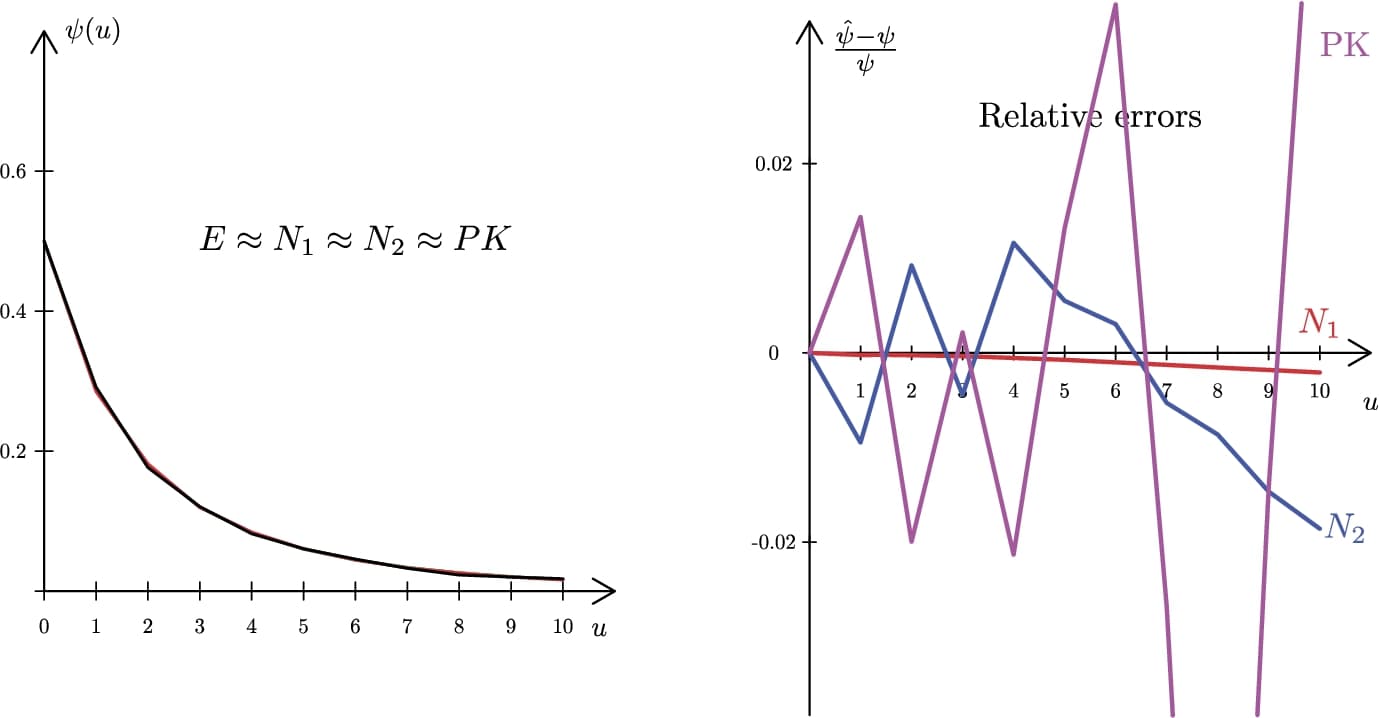
The key takeaway is that for large surpluses, $\psi (u)$ is not just bounded by an exponential function, it behaves like one. The image below shows plots of the ruin probability $\psi (u)$ (black curve) alongside several approximations. Notice how closely they track the true function, especially for larger values of $u$. The right panel shows the relative errors of these approximations, highlighting that more sophisticated approximations like Cramér-Lundberg can offer significant improvements in accuracy over the basic Lundberg bound.

Practical Application: Capital Requirements

The most important application of these results is determining the capital an insurer needs to hold. We can use Lundberg's inequality to find the minimum initial surplus $u$ required to keep the probability of ruin below a certain tolerance level, $\beta$.

We want $\psi (u)\le \beta$. Using Lundberg's inequality, it is sufficient to ensure:

Solving for $u$ gives:

This simple formula creates a direct trade-off between the desired security level ($\beta$), the portfolio's riskiness ($R$), and the required capital ($u$).

Let's see this in action.

Example: Capital for a Target Ruin Probability

An insurer models its annual aggregate claims as approximately Normal with a mean of $10M and a standard deviation of $4M. Its annual premium income is $11M. From this, the adjustment coefficient is approximated as $R\approx 0.0125$. (This comes from approximating the surplus process with Brownian motion, where $R=2{\mu }_{surplus}/{\sigma }_{surplus}^2$).

The board wants to hold enough capital to ensure the probability of ultimate ruin is less than 1%. How much initial surplus is required?

1. Parameters:

   • Target ruin probability $\beta =0.01$.
   • Adjustment coefficient $R=0.0125$.

2. Calculate Required Surplus (u):

   $$u\ge \frac{\ln (1/\beta )}{R}=\frac{\ln (1/0.01)}{0.0125}=\frac{\ln (100)}{0.0125}\approx \frac{4.605}{0.0125}=368,400$$

   The insurer must hold an initial surplus of at least $368,400 to meet its risk tolerance, based on this model and the conservative Lundberg bound. Using the Cramér-Lundberg approximation would yield a slightly lower, but more complex, value. For regulatory purposes, the simpler, more conservative bound is often preferred.

Conclusion

In this lesson, you have learned how to apply the adjustment coefficient, connecting its calculation to the fundamental goal of quantifying insolvency risk. We have moved from the abstract definition of $R$ to its practical use in estimating one of the most important metrics in actuarial science.

Key Takeaways:

• Lundberg's inequality, $\psi (u)\le e^{-Ru}$, provides a simple and robust upper bound on the probability of ultimate ruin. It is a cornerstone of classical ruin theory.
• The Cramér-Lundberg approximation, $\psi (u)\approx C{e}^{-Ru}$, offers a more precise estimate for large initial surpluses, acknowledging that the true probability is slightly less than the bound but follows the same exponential decay.
• For the special case of exponential claims, the ruin probability is known exactly: $\psi (u)=\frac{1}{1+\theta }{e}^{-Ru}$.
• A key practical application is calculating the required initial surplus $u$ to keep the ruin probability below a target level $\beta$, using the formula $u\ge \ln (1/\beta )/R$.

Preview of the Next Lesson

So far in our study of ruin theory, we have focused on models with continuous claim amounts and have relied on bounds and approximations. In the next lesson, we will shift gears to a different scenario: where claim amounts are discrete values. We will learn a powerful recursive method that allows for the exact calculation of the ultimate ruin probability in such cases, providing a valuable contrast to the estimation techniques we've covered today.