Transition Probabilities from Generator Matrix

Introduction

In our previous lesson, we established that the evolution of transition probabilities $P (t)$ in a continuous-time Markov process is governed by the Kolmogorov forward and backward differential equations, $P^{'} (t) = P (t) Q$ and $P^{'} (t) = QP (t)$ . We also solved these equations for a simple three-state model by tackling the system of ordinary differential equations (ODEs) one by one.

Today, we will introduce a more direct and powerful method to solve this system for any time-homogeneous process: matrix exponentiation. Just as the solution to the simple scalar differential equation $p^{'} (t) = q p (t)$ is $p (t) = e^{q t}$ , we will see that the solution to the matrix differential equation $P^{'} (t) = P (t) Q$ is $P (t) = e^{t Q}$ . This lesson will focus on defining this matrix exponential and, more importantly, on the practical techniques for calculating it. This approach allows us to find all transition probabilities simultaneously, a significant advantage for models with many states.

The Matrix Exponential Solution

Let's begin by formalizing the solution to the Kolmogorov equations. The derivation involves starting from the Chapman-Kolmogorov relation in continuous time, $P (t + δ t) = P (t) P (δ t)$ , and taking the limit as $δ t \to 0$ . This process leads directly to the forward differential equation.

The following video walks through this derivation and then introduces the matrix exponential as the solution, drawing a clear parallel to the familiar scalar case.

continuous time markov

This video from Gareth Tribello, titled "continuous time markov", provides an excellent derivation of the forward equation and introduces its solution via matrix exponentiation.

Please watch from the beginning of the derivation at this point, which recaps the Chapman-Kolmogorov relation and derives the forward equation, \mathbf{P}'(t) = \mathbf{P}(t)\mathbf{Q}. Then, continue watching the crucial next segment from this part, where the lecturer explains that the solution is the matrix exponential, \mathbf{P}(t) = e^{t\mathbf{Q}}, and defines it using its Taylor series expansion: \mathbf{P}(t) = e^{t\mathbf{Q}} = \sum_{k=0}^{\infty} \frac{(t\mathbf{Q})^k}{k!} = \mathbf{I} + t\mathbf{Q} + \frac{t^2\mathbf{Q}^2}{2!} + \frac{t^3\mathbf{Q}^3}{3!} + \dots Pay close attention to the distinction made: this is not the same as taking the exponential of each element in the matrix.

The key takeaway is that the entire matrix of transition probabilities at time $t$ , $P (t)$ , can be found by computing the exponential of the matrix $t Q$ .

Calculating the Matrix Exponential

While the infinite series definition is fundamental, it is not a practical way to compute $P (t)$ . A much more efficient method relies on the diagonalization of the generator matrix $Q$ .

If the $n \times n$ generator matrix $Q$ has $n$ distinct eigenvalues, it can be diagonalized as:
$Q = AD A^{- 1}$
where:

$D$ is a diagonal matrix whose entries are the eigenvalues of $Q$ , $(λ_{1}, λ_{2}, \dots, λ_{n})$ .
$A$ is a matrix whose columns are the corresponding right-eigenvectors of $Q$ .
$A^{- 1}$ is the inverse of the eigenvector matrix.

Using this decomposition, the matrix exponential can be calculated as:
$P (t) = e^{t Q} = A e^{t D} A^{- 1}$
The term $e^{t D}$ is straightforward to compute, as the exponential of a diagonal matrix is simply the diagonal matrix of the exponential of its elements:
$e^{t D} = diag (e^{t λ_{1}}, e^{t λ_{2}}, \dots, e^{t λ_{n}})$
This powerful result reduces the problem of computing a matrix exponential to the more familiar tasks of finding eigenvalues, eigenvectors, and a matrix inverse.

The following resource formally presents this method.

[PDF] A Sensitivity Analysis of the Premiums for a Permanent Health ...

This paper by Rickayzen, though focused on a larger application, contains a concise summary of the mathematical model for transition probabilities.

In the section "2 The Model", please read the subsection "The Chapman-Kolmogorov backward system". Focus on equations (5), (6), (7), and (8). These equations lay out the logic we just discussed: the differential equation (5) has the matrix exponential solution (6), which can be practically computed via diagonalization using equation (8).

Worked Example: A Three-State Model

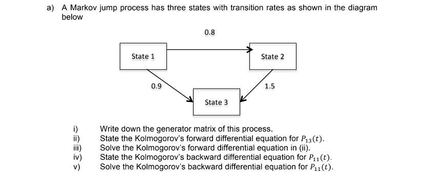
Let's apply this technique to compute the transition probability matrix for a concrete example. Consider the three-state Markov jump process shown in the diagram below.

A three-state Markov jump process with transitions from State 1 to States 2 and 3, and from State 2 to State 3. State 3 is an absorbing state.

Step 1: Construct the Generator Matrix Q

From the diagram, we have the following transition rates:

$q_{12} = 0.8$
$q_{13} = 0.9$
$q_{23} = 1.5$

All other off-diagonal rates are zero. The diagonal elements are the negative sum of the rates out of each state:

$q_{11} = - (q_{12} + q_{13}) = - (0.8 + 0.9) = - 1.7$
$q_{22} = - q_{23} = - 1.5$
$q_{33} = 0$ (State 3 is absorbing)

This gives us the generator matrix:

Q = - 1.7 00 0.8 - 1.5 0 0.9 1.5 0

Step 2: Find Eigenvalues and Eigenvectors

Since $Q$ is an upper triangular matrix, its eigenvalues are simply the diagonal entries:
$λ_{1} = - 1.7, λ_{2} = - 1.5, λ_{3} = 0$
These are distinct, so the matrix is diagonalizable. Next, we find the corresponding right-eigenvectors by solving $(Q - λ_{i} I) v_{i} = 0$ for each eigenvalue.

For $λ_{1} = - 1.7$ , we find the eigenvector $v_{1} = (1, 0, 0)^{T}$ .
For $λ_{2} = - 1.5$ , we find the eigenvector $v_{2} = (4, 1, 0)^{T}$ .
For $λ_{3} = 0$ , we find the eigenvector $v_{3} = (1, 1, 1)^{T}$ .

The matrix of eigenvectors $A$ and its inverse $A^{- 1}$ are:

A = 100410111 and A^{- 1} = 100 - 4 10 3 - 1 1

Step 3: Assemble the Solution

Now we can compute $P (t) = A e^{t D} A^{- 1}$ . The diagonal matrix of exponentiated eigenvalues is:

e^{t D} = e^{- 1.7 t} 00 0 e^{- 1.5 t} 0 00 e^{0 t} = e^{- 1.7 t} 00 0 e^{- 1.5 t} 0 001

Performing the matrix multiplication $A (e^{t D} A^{- 1})$ gives us the final transition probability matrix:

P (t) = e^{- 1.7 t} 00 - 4 e^{- 1.7 t} + 4 e^{- 1.5 t} e^{- 1.5 t} 0 3 e^{- 1.7 t} - 4 e^{- 1.5 t} + 1 1 - e^{- 1.5 t} 1

This matrix gives us every transition probability $p_{ij} (t)$ for any time $t$ . For example, the probability of being in State 2 at time $t$ , having started in State 1, is $p_{12} (t) = 4 e^{- 1.5 t} - 4 e^{- 1.7 t}$ .

This example demonstrates how a systematic, algebraic process can solve for the entire system's dynamics at once, fulfilling the goal of this lesson.

Conclusion

In this lesson, we have moved from solving Kolmogorov's equations one at a time to finding a general solution for the entire transition probability matrix, $P (t)$ .

Key Takeaways:

The solution to the Kolmogorov differential equations ( $P^{'} (t) = QP (t)$ or $P^{'} (t) = P (t) Q$ ) for a time-homogeneous process is given by the matrix exponential: $P (t) = e^{t Q}$ .
The matrix exponential is defined by the infinite Taylor series $\sum_{k = 0}^{\infty} \frac{( t Q ) ^{k}}{k !}$ .
The most practical method for calculating the matrix exponential is through diagonalization: $P (t) = A e^{t D} A^{- 1}$ , where $A$ is the matrix of eigenvectors and $D$ is the diagonal matrix of eigenvalues of $Q$ .
This method allows us to derive an explicit formula for every transition probability $p_{ij} (t)$ simultaneously.

With this powerful tool in hand, we are now equipped to analyze the financial implications of movements between states. In our next lesson, we will use these transition probabilities to calculate the expected present value of state-contingent cash flows, a foundational concept for pricing and reserving in life and health insurance.

Recommended resources

Introduction

The Matrix Exponential Solution

Calculating the Matrix Exponential

Worked Example: A Three-State Model

Conclusion