Crude Mortality Rate Graduation

The Rationale for Graduating by Reference

Populations often share a similar shape of mortality, even if the overall level of mortality differs. For instance, a group of insured individuals and the general population both experience mortality rates that are low at young ages, rise slightly in early adulthood, and then increase exponentially at older ages. However, the insured group might have consistently lower mortality at every age.

Graduation by reference leverages this idea. We start with a "standard table"—a mortality table based on a large, reliable dataset like a national census or a massive insurance portfolio—and assume our population's true mortality rates can be expressed as a simple transformation of the rates in that standard table.

This approach is particularly useful when:

• Our own dataset is small or sparse, leading to volatile crude rates.
• We lack sufficient data at very young or very old ages.
• We believe the underlying mortality pattern of our group is similar in shape to a larger, well-documented population.

The general process involves three steps:

1. Select a standard table that is a plausible baseline for the population being studied.
2. Propose a linking function that mathematically connects the mortality rates of the standard table to the rates of our population.
3. Estimate the parameters of this linking function using the observed data (deaths and exposures), typically via maximum likelihood estimation.

Linking Functions: The Bridge Between Tables

The linking function defines the mathematical relationship between our graduated force of mortality, ${\mu }_x^o$, and the force of mortality from the standard table, ${\mu }_x^s$. The choice of function depends on how we believe our population's mortality deviates from the standard.

Some common linking functions include:

• A constant scaling factor:

  $${\mu }_x^o=a\cdot {\mu }_x^s$$

  This is the simplest model, assuming our population's mortality is just a fixed percentage of the standard table's mortality across all ages.

• A linear transformation:

  $${\mu }_x^o=a+b\cdot {\mu }_x^s$$

  This provides more flexibility, allowing for both a multiplicative ($b$) and an additive ($a$) adjustment.

• An age-dependent scaling factor:

  $${\mu }_x^o=(a+bx)\cdot {\mu }_x^s$$

  This sophisticated model allows the relationship to change with age. For example, the mortality advantage of a certain group might diminish as they get older, a feature this model can capture.

• An exponential adjustment:

  $${\mu }_x^o={\mu }_x^s\cdot \exp (a+bx)$$

  This is a very common and effective model. By taking logarithms, the relationship becomes linear: $\ln ({\mu }_x^o)=\ln ({\mu }_x^s)+a+bx$. This implies that the log difference in mortality between the two populations is a linear function of age.

The following reading discusses some of these simple adjustments in a practical context.

A Practical Case Study: Choosing the Best Model

Once we have our candidate standard tables and linking functions, how do we select the best combination? As in the previous lesson, we fit each model using Maximum Likelihood Estimation (assuming Poisson-distributed deaths) and then compare them using statistical criteria like AIC, BIC, or simply the maximized log-likelihood value.

The following thesis provides a complete, real-world example of this process for an insurance portfolio.

This case study perfectly illustrates the graduation-by-reference workflow: proposing multiple models, fitting them to data, and using statistical evidence to select the most appropriate one.

A Broader Perspective: Direct and Indirect Standardization

The methods we are discussing are part of a wider family of techniques known as standardization, which are central to epidemiology and public health for making fair comparisons between populations with different structures (e.g., different age distributions). The two main approaches are indirect and direct standardization.

The following video provides an excellent and clear explanation of both concepts.

The graduation-by-reference technique we have focused on is a sophisticated form of direct standardization. We are essentially creating an age-adjusted mortality table for our population by "borrowing" the smooth age pattern from a standard table.

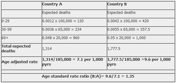
The image below shows a simple calculation of an age-adjusted rate and an age-standardized rate ratio, which is a comparison of these adjusted rates (e.g., Country B's rate / Country A's rate). This exemplifies the direct method described in the video.

Conclusion

In this lesson, we have added a crucial and flexible tool to our graduation toolkit. Parametric formulas are powerful when a known law of mortality applies, but graduating by reference to a standard table offers a practical and robust alternative when data is sparse or the underlying mortality pattern is less certain.

Key Takeaways:

• Graduation by Reference: This method adjusts a pre-existing, reliable standard mortality table to fit the observed data of a smaller population.
• Process: It involves selecting a standard table, defining a mathematical linking function, and estimating the function's parameters using Maximum Likelihood Estimation.
• Linking Functions: Common forms include constant scaling, linear transformations, and exponential adjustments, which offer varying degrees of flexibility.
• Model Selection: The best combination of standard table and linking function is chosen by comparing statistical metrics like AIC, BIC, and log-likelihood across different models.
• Standardization Context: This technique is a form of direct standardization, a method used to create comparable rates by removing the confounding effect of population structure. The related concept of indirect standardization yields the Standardised Mortality Ratio (SMR), a single summary measure of relative mortality risk.

Preview of the Next Lesson

We have now covered parametric methods and semi-parametric methods (by reference). What if we want even more flexibility and wish to let the data "speak for itself" as much as possible? In our next lesson, we will explore graphical and spline-based methods. These techniques impose even fewer structural assumptions, aiming to produce a smooth curve that follows the data's contours very closely, a process that relies heavily on visual judgment and non-parametric smoothing techniques.