Comparing LLM Activation Functions: SwiGLU vs. GeLU

Introduction

Welcome back. In our last lesson, we focused on the attention sub-layer, exploring how Grouped-Query Attention (GQA) and Multi-Query Attention (MQA) optimize the KV-cache to make inference more efficient. We saw how these architectural changes dramatically reduce memory bandwidth, a critical bottleneck for deploying LLMs.

Today, we shift our focus to the other major component within a Transformer block: the Position-wise Feed-Forward Network (FFN). While attention handles information mixing across the sequence, the FFN is responsible for much of the model's deep computational work at each position. The choice of activation function inside this network is a crucial design decision that has evolved significantly from the original Transformer.

This lesson will address the learning outcome: Compare different activation functions used in modern LLMs, such as SwiGLU and GeLU. We will trace the progression from the classic ReLU, understand its limitations, and then dive into the smoother, more powerful functions that are standard in today's state-of-the-art models.

From ReLU's Simplicity to its Limitations

Every FFN in a Transformer block consists of two linear transformations with a non-linear activation function in between. This non-linearity is essential; without it, the FFN would just be a single, larger linear layer, severely limiting the model's expressive power.

For years, the Rectified Linear Unit (ReLU), defined as $ReLU (x) = max (0, x)$ , was the default choice in deep learning due to its simplicity and computational efficiency. However, it has notable drawbacks that become more pronounced in deep Transformer architectures.

To understand these limitations and set the stage for modern alternatives, please read the first part of the following article.

Choice of Activation Functions (ReLU, GeLU, SwiGLU)

This article provides a clear overview of the role of activation functions in the FFN and the pros and cons of the foundational choice, ReLU.

Please read the introduction and the section on 'Rectified Linear Unit (ReLU)'. Focus on understanding the 'dying ReLU' problem and why its non-smooth nature can be a disadvantage.

As you read, the key takeaway is that ReLU's hard-zeroing of all negative inputs can cause neurons to "die" and stop learning entirely. This led researchers to seek smoother activation functions that could mitigate this issue while retaining good performance.

GeLU: A Smoother, Probabilistic Approach

The first major successor to ReLU in Transformer models like BERT and the early GPT series was the Gaussian Error Linear Unit (GeLU). GeLU introduces a smoother curve and avoids the "dying neuron" problem by allowing small negative values to pass through.

The core intuition behind GeLU is probabilistic: it weights an input by its value, but this weighting is modulated by the probability that it is greater than other inputs drawn from a standard normal distribution. This is mathematically expressed as:

$GeLU (x) = x \cdot Φ (x)$

where $Φ (x)$ is the cumulative distribution function (CDF) of the standard Gaussian distribution.

The following video provides an excellent explanation of GeLU, from its motivation and mathematical underpinnings to its practical benefits.

GELU Activation Function in the LLM Architecture

This video from Vizuara breaks down why GeLU was developed as an improvement over ReLU and how it functions.

Please watch from 04:20 to 10:57. The first part (until 07:30) contrasts ReLU's limitations with GeLU's mathematical form. The second part (from 09:44) summarizes the key advantages that made GeLU a standard in many foundational LLMs.

In summary, GeLU's main advantages over ReLU are:

Smoothness: It is differentiable everywhere, which can lead to better and more stable optimization during training.
Avoids Dead Neurons: It does not zero out all negative inputs, allowing gradients to flow and learning to continue even for neurons that receive negative inputs.

SwiGLU: The Gated Revolution

While GeLU was a significant improvement, the latest generation of top-performing models, including Llama, Mistral, and PaLM, has converged on an even more powerful approach: variants of the Gated Linear Unit (GLU), most notably SwiGLU.

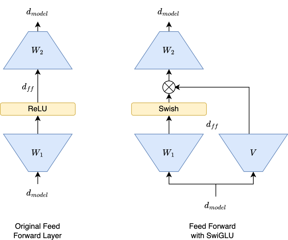
SwiGLU isn't just a new activation function; it's a change to the FFN's architecture itself. It introduces a gating mechanism, where the network learns to dynamically control the flow of information.

Comparison of Original Feed-Forward Layer with SwiGLU Feed-Forward Layer — This diagram illustrates the structural difference. A standard ReLU FFN (left) is a simple sequence. The SwiGLU FFN (right) uses two parallel linear projections, where one path 'gates' the other through element-wise multiplication, providing more expressive power.

To understand this concept, let's start with a foundational explanation of gating.

Gated Linear Units: The FFN Architecture Behind Modern LLMs

This article by Michael Brenndoerfer provides a fantastic deep dive into Gated Linear Units. We'll start with the high-level intuition behind the gating mechanism.

Please read the first two sections: 'Gated Linear Units' and 'The Gating Mechanism'. This will explain the core idea of using multiplicative interactions to increase the network's expressiveness.

Now that you understand the concept of gating, let's look at the specific implementation in SwiGLU. The SwiGLU FFN uses three weight matrices and is defined as:

$FFN_{SwiGLU} (x) = (Swish (x W_{1}) \otimes (x V)) W_{2}$

Where:

$x$ is the input.
$W_{1}$ , $V$ , and $W_{2}$ are learnable weight matrices.
$\otimes$ denotes element-wise multiplication.
Swish is an activation function defined as $Swish (x) = x \cdot σ (x)$ , where $σ$ is the sigmoid function. Notice its self-gating nature.

Let's watch a concise explanation of SwiGLU as it's used in the Llama architecture.

LLaMA explained: KV-Cache, Rotary Positional Embedding, RMS Norm, Grouped Query Attention, SwiGLU

This clip from Umar Jamil's video on Llama provides a practical look at the SwiGLU function, connecting it back to the original research paper.

Watch from 01:04:05 to 01:08:15. The video explains the structure of the SwiGLU FFN, the underlying Swish (or SiLU) function, and the empirical evidence for its superior performance.

The key insight is that the gating mechanism allows for much richer, input-dependent transformations. The network can learn to selectively pass, block, or scale information for each feature, which has proven to be highly effective in practice.

The Engineer's View: Parameter Trade-offs

Your goal is to be a top-tier engineer, and a crucial part of that is understanding the trade-offs in model design. The move to SwiGLU is not free; it impacts the model's parameter count.

A standard FFN has two weight matrices: $W_{1}$ (expanding to d_ff) and $W_{2}$ (contracting to d_model).
A SwiGLU FFN has three weight matrices: $W_{1}$ and $V$ (both expanding to d_ff), and $W_{2}$ (contracting to d_model).

This means that for the same hidden dimension (d_ff), a SwiGLU FFN has more parameters. To maintain a comparable parameter count to a standard FFN, modern models like Llama adjust the hidden dimension.

The following reading explains this trade-off and the common solution.

Gated Linear Units: The FFN Architecture Behind Modern LLMs

Let's return to the Brenndoerfer article to understand the practical implications of using SwiGLU on the model's size.

Read the section 'Parameter Efficiency Analysis'. It provides a clear derivation showing why the hidden dimension d_ff in a SwiGLU network is often set to around 2/3 of the size used in a standard FFN to keep the parameter count the same.

This 2/3 scaling factor for the hidden dimension is a critical piece of practical knowledge when analyzing or designing modern LLM architectures.

Test your understanding!

A standard Transformer model uses d_model = 4096 and a d_ff = 4 * d_model = 16384 with a ReLU activation. You want to build a new model with a SwiGLU FFN that has roughly the same number of parameters in its FFN layers.

What should the d_ff of your new SwiGLU-based model be?

Show answer

To maintain parameter parity, the new hidden dimension (d_ff') should be approximately 2/3 of the original:

d_ff' ≈ (2/3) * d_ff
d_ff' ≈ (2/3) * 16384
d_ff' ≈ 10922.67

Since hidden dimensions are typically chosen to be multiples of 64, 128, or 256 for hardware efficiency, a practical choice would be around 11008 (which is a multiple of 256, as used in Llama models).

Comparison and Summary

Let's bring everything together. The evolution from ReLU to GeLU to SwiGLU is a story of moving from simplicity to smoothness and finally to dynamic, gated expressiveness.

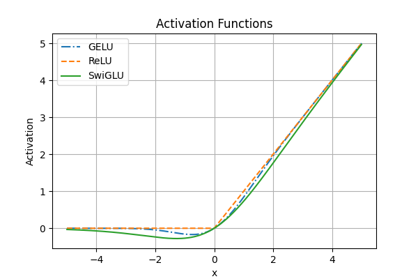
Comparison of Activation Functions: GELU, ReLU, and SwiGLU — This plot visually summarizes the functions we've discussed. ReLU's sharp corner at zero is contrasted with the smooth curves of GeLU and Swish (the basis for SwiGLU). Note how GeLU and Swish dip slightly below zero, a key difference from ReLU.

Here is a summary table comparing the three activation functions:

Feature	ReLU	GeLU	SwiGLU (in an FFN)
Mathematical Form	`max(0, x)`	`x * Φ(x)` (often approximated)	`(Swish(xW) ⊗ xV)W₂`
Smoothness	No (non-differentiable at 0)	Yes (differentiable everywhere)	Yes (differentiable everywhere)
"Dying Neuron" Problem	Suffers from it	Avoids it	Avoids it
Architecture	Standard FFN	Standard FFN	Gated FFN with 3 weight matrices
Key Advantage	Computationally very cheap	Good balance of performance and cost	Highest performance via dynamic, learned gating
Commonly Found In	Older CNNs/Transformers	BERT, GPT-2, Falcon	Llama, Mistral, PaLM, GPT-3.5/4 class models

Conclusion

In this lesson, you've explored the evolution of activation functions within the Transformer's feed-forward network. This is a perfect illustration of how deep learning research progresses: identifying a limitation (dying ReLUs), proposing a smoother alternative (GeLU), and finally developing a more expressive and powerful architecture (SwiGLU) that becomes the new standard.

Key Takeaways:

ReLU is simple and fast but its hard-zeroing can impede learning ("dying neurons").
GeLU provides a smooth, probabilistic alternative that avoids the dead neuron problem and was a standard for many foundational LLMs.
SwiGLU represents a more advanced, gated architecture. It allows the network to dynamically control information flow, leading to superior performance in modern LLMs.
This performance comes with a parameter trade-off, which is managed by adjusting the FFN's hidden dimension to maintain a similar parameter budget.

What's Next?

You have now examined key architectural components and optimizations of modern LLMs, including Rotary Positional Embeddings (RoPE), KV-caching, Grouped-Query Attention (GQA), and now advanced activation functions like SwiGLU.

In the next lesson, we will synthesize this knowledge to analyze and compare the architectural choices of leading open-weight (Llama 3, Mistral) and proprietary (GPT-4, Claude 3) models. You'll see how these different building blocks are combined to create the models that define the state of the art.

Recommended resources