Introduction
Welcome to your next lesson. In our previous session, you learned how to extract and visualize the [sequence_length x sequence_length] attention matrix to interpret a model's focus. That square matrix is not just a tool for interpretability; it's also the root of the Transformer's most significant computational challenge.
Today, we will dissect that challenge. The learning outcome is to explain the quadratic complexity of self-attention with respect to sequence length. We will move from the visual representation of the attention matrix to a formal analysis of its computational and memory costs. Understanding this "attention bottleneck" is fundamental. It is the primary constraint that has driven years of research into the more efficient architectures that power today's leading-edge models.
1. The Source of Quadratic Scaling: Every Token Attends to Every Other
At its core, the reason for quadratic complexity is simple and intuitive. For a sequence of length n, self-attention is designed to calculate the relationship between every possible pair of tokens.
- Token 1 needs to be compared with tokens 1, 2, 3, ...,
n. - Token 2 needs to be compared with tokens 1, 2, 3, ...,
n. - ...
- Token
nneeds to be compared with tokens 1, 2, 3, ...,n.
This all-to-all comparison results in n * n = n² interactions. This is visually represented by the n x n attention matrix you worked with in the last lesson.
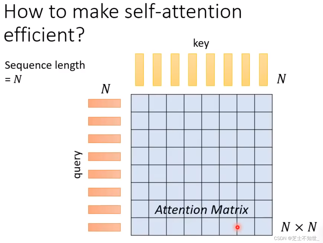
To build on this intuition, the following short video provides an excellent conceptual walkthrough of how these n² interactions arise from the dot products of query and key vectors.
Linformer: Self-Attention with Linear Complexity (Paper Explained)
In this clip from Yannic Kilcher's explanation of the Linformer paper, he provides a clear, high-level overview of why standard self-attention has N-squared complexity. Focus on the analogy of routing information between tokens.
Watch the segment from 01:46 to 04:53. Pay attention to how the need to compute an inner product for every query-key pair naturally leads to an n-squared operation count.
This conceptual understanding provides the foundation. Now, let's formalize it by analyzing the specific mathematical operations involved.
2. A Formal Complexity Analysis
The total cost of self-attention comes from a three-stage pipeline. The most comprehensive way to understand this is to break down the complexity of each stage. The following article provides a clear, step-by-step analysis with concrete mathematical derivations.
Attention Complexity: Quadratic Scaling, Memory Limits & Efficient ...
The article 'Attention Complexity' by Michael Brenndoerfer offers a detailed breakdown of the computational and memory costs of self-attention. It's an excellent resource for a rigorous understanding.
Please read the sections titled 'The Quadratic Bottleneck' and 'The Three-Stage Computation Pipeline' (from the start up to, but not including, 'Putting It Together'). Focus on how the author derives the complexity for each of the three stages: computing scores, applying softmax, and computing outputs.
As you've just read, the total complexity arises from summing the costs of the three main stages. Let's summarize the key findings, using n for sequence length and d for the model's hidden dimension (specifically, the dimension of the key/value vectors, d_k and d_v).
-
Stage 1: Score Computation (
S = QK^T)- This is a matrix multiplication between
Q(shapen x d_k) andK^T(shaped_k x n). - The result is the
n x nattention score matrixS. - The number of floating-point operations (FLOPs) is proportional to
n * n * d_k. - Complexity:
O(n²d). This is the first major quadratic operation.
- This is a matrix multiplication between
-
Stage 2: Normalization (
softmax(S))- The softmax function is applied to each of the
nrows of the score matrix. - Each row has
nelements, so the cost per row isO(n). - Total cost for
nrows isn * O(n). - Complexity:
O(n²). While quadratic, this cost is typically much smaller than the matrix multiplications whendis large.
- The softmax function is applied to each of the
-
Stage 3: Output Computation (
Output = softmax(S)V)- This is a matrix multiplication between the
n x nattention weights andV(shapen x d_v). - The result is the final output matrix of shape
n x d_v. - The number of FLOPs is proportional to
n * n * d_v. - Complexity:
O(n²d). This is the second major quadratic operation.
- This is a matrix multiplication between the
Summing these gives a total time complexity of O(n²d). This formula makes the trade-offs clear: the cost grows quadratically with sequence length n, but only linearly with the model dimension d.
Test your understanding!
Imagine a single attention layer takes 2 seconds to process a sequence of 2048 tokens on a specific GPU. Based on the O(n²) scaling with respect to sequence length, approximately how long would you expect it to take to process a sequence of 8192 tokens?
Show answer
The sequence length increases by a factor of 8192 / 2048 = 4.
Since the complexity is quadratic with sequence length, the computation time should increase by a factor of 4² = 16.
Therefore, the estimated time would be 2 seconds * 16 = 32 seconds. This demonstrates the explosive growth in computation as context windows get longer.
3. The Memory Bottleneck: It's Not Just About FLOPs
While the O(n²d) time complexity is significant, in practice, the even bigger constraint is often memory. The reason is the same: the n x n attention matrix.
-
Memory Complexity: To perform the calculations, the GPU must materialize and store the
n x nattention score matrix. Storing this matrix requiresO(n²)space. -
Practical Impact: Using standard 32-bit floating-point numbers (4 bytes), an attention matrix for a sequence of 8192 tokens requires
8192 * 8192 * 4 bytes ≈ 268 MBof GPU memory. For a 16-head attention mechanism, this becomes16 * 268 MB ≈ 4.3 GB. This is for just one layer in the model and only for the attention weights themselves, not including model parameters, gradients, or other activations. As you can see, memory consumption quickly becomes prohibitive.
Furthermore, a crucial insight for an engineer aiming for elite proficiency is that the true bottleneck is often memory bandwidth, not just memory capacity or raw FLOPs.
MedAI #54: FlashAttention: Fast and Memory-Efficient Exact Attention with IO-Awareness | Tri Dao
This talk on FlashAttention by one of its creators, Tri Dao, provides an expert's perspective. It highlights why the naive attention implementation is slow, focusing on the distinction between computation and memory access.
Please watch two short segments: 08:02 - 10:06: This part recaps the quadratic compute and memory complexity, reinforcing what we've just discussed. 10:06 - 12:02: This is the key segment. Focus on the argument that the true bottleneck is not computation (FLOPs) but memory reads/writes from the slow, large GPU memory (HBM).
The core takeaway from the video is profound: modern GPUs can perform calculations (FLOPs) much faster than they can move data from their main memory (HBM) to the on-chip processing units (SRAM). Because the standard attention algorithm requires writing the entire n x n matrix to HBM and then reading it back, it is I/O-bound, not compute-bound. This means the model spends most of its time waiting for data to move, not actually doing math. This is the problem that efficient attention mechanisms like FlashAttention were designed to solve.
4. Perspective: Attention vs. RNN Complexity
To fully appreciate the trade-offs, it's useful to compare self-attention's complexity to that of the Recurrent Neural Networks (RNNs) you studied in Module 1.
The article you read earlier contains a section that does exactly this.
Attention Complexity: Quadratic Scaling, Memory Limits & Efficient ...
Let's return to the 'Attention Complexity' article. The author provides a concise comparison between the scaling properties of attention and RNNs.
Please read the section 'Attention vs. RNN Complexity'. Note the complexity formulas for both architectures and the analysis of the 'crossover point'.
Here is a summary of the comparison:
| Architecture | Time Complexity | Scaling with Sequence Length (n) | Scaling with Dimension (d) | Parallelizability |
|---|---|---|---|---|
| Self-Attention | O(n²d) |
Quadratic | Linear | High (per-layer) |
| RNN | O(nd²) |
Linear | Quadratic | Low (sequential) |
This table reveals a critical trade-off. For a typical model where n > d (e.g., sequence length 4096, dimension 1024), attention is computationally more expensive than an RNN. However, the operations within an attention layer can be massively parallelized across the sequence length n, which is a perfect fit for modern GPUs. In contrast, RNNs must process the sequence token by token, creating a sequential bottleneck that hardware cannot overcome. This parallel nature is why Transformers replaced RNNs for most state-of-the-art sequence modeling, despite the quadratic complexity.
Conclusion
In this lesson, you have rigorously analyzed the computational and memory profile of the self-attention mechanism. This understanding is not just academic; it directly informs model design, hardware selection, and the practical limits of what can be achieved with standard Transformer architectures.
Key Takeaways:
- Self-attention has a time complexity of
O(n²d)and a memory complexity ofO(n²), both of which are quadratic in sequence lengthn. - This quadratic scaling arises from the all-to-all comparison required to compute the
n x nattention matrix. - In practice, memory consumption and memory bandwidth (I/O) are often the primary bottlenecks, making attention I/O-bound on modern hardware.
- Compared to RNNs (
O(nd²)), attention scales poorly with sequence length but scales better with model dimension and is highly parallelizable, which is why it dominates modern NLP.
What's Next?
You now have a deep understanding of the problem. In the next lesson, we will begin exploring the solutions. We will describe the core ideas behind efficient attention variants like FlashAttention and sparse attention, which are clever algorithms designed to overcome the quadratic bottleneck while preserving the power of the attention mechanism. This will lead us directly into the architectural innovations that make today's long-context models possible.