Layer Normalization: Stabilizing Transformer Training

Introduction

In our last lesson, we explored the position-wise feed-forward network (FFN), the second major sub-layer in a Transformer block. We established that its role is to introduce non-linearity, processing each token's representation independently after the self-attention mechanism has mixed information across the sequence.

You may recall that both the attention and FFN sub-layers are wrapped in what the original paper calls an "Add & Norm" step. We've seen how the residual "Add" connection helps with gradient flow, but we haven't yet addressed the "Norm" part. Without it, training deep networks like Transformers would be practically impossible.

Today's learning outcome is to implement layer normalization and explain its importance for stabilizing training in deep transformers. We will dissect what Layer Normalization does, why it's preferred over other normalization techniques like Batch Normalization for sequence data, and explore a crucial architectural choice: its placement within the Transformer block.

The Challenge of Training Deep Networks

As we stack dozens of Transformer blocks to create a deep model, the outputs of each layer—the activations—are fed as inputs into the next. Without any constraints, the scale of these activations can vary wildly. They can grow exponentially, leading to exploding gradients and unstable training, or shrink to near zero, causing gradients to vanish and learning to stall.

This problem, known as internal covariate shift, is what normalization techniques are designed to solve. They control the distribution of activations (mean and variance) to ensure a more stable and efficient optimization process.

Your experience with GLMs gave you a foundation in how feature scaling can be important for model convergence. In deep learning, this concept is taken a step further by normalizing the internal activations between layers. A common method is Batch Normalization, but it has drawbacks for NLP tasks.

In short, Batch Normalization's reliance on batch statistics makes it ill-suited for the variable sequence lengths and often small batch sizes common in training large language models.

Layer Normalization: Normalizing Across Features

Layer Normalization (LayerNorm) offers an elegant solution. Instead of normalizing across the batch dimension, it normalizes across the feature dimension for each training example independently.

In a Transformer, this means that for each token in the sequence, we normalize its embedding vector. The calculation is done independently for every single token.

The Mathematics of LayerNorm

For a given input vector $x$ (representing a single token's embedding), the process is:

1. Calculate Mean and Variance: Compute the mean $\mu$ and variance ${\sigma }^2$ of the elements within that single vector $x$.

   $$\mu =\frac{1}{H}\sum _{i=1}^H{x}_i\text{and}{\sigma }^2=\frac{1}{H}\sum _{i=1}^H(x_i-\mu {)}^2$$

   where $H$ is the number of features (i.e., the embedding dimension, $d_{\text{model}}$).

2. Normalize: Use the calculated mean and variance to normalize the input vector.

   $$\hat{x}=\frac{x-\mu }{\sqrt{{\sigma }^2+ϵ}}$$

   The small constant $ϵ$ (e.g., $10^{-5}$) is added for numerical stability to prevent division by zero.

3. Scale and Shift: Apply two learnable parameter vectors, a gain ($\gamma$) and a bias ($\beta$), to the normalized output.

   $$\text{LayerNorm}(x)=\gamma \odot \hat{x}+\beta$$

   These parameters allow the model to scale and shift the normalized output. This is crucial because it gives the network the flexibility to learn if and how much normalization is actually needed. The network can learn to effectively "undo" the normalization by setting $\gamma$ to $\sqrt{{\sigma }^2}$ and $\beta$ to $\mu$, preserving its expressive power.

To see this process with concrete numbers, the following video provides an excellent walkthrough.

An Implementation From Scratch

Given your background, seeing this implemented from scratch can solidify the concept. Andrej Karpathy's "Let's build GPT" video includes a brilliant segment where he first builds LayerNorm from basic PyTorch operations before using the built-in nn.LayerNorm.

Here's what a clean, standalone PyTorch implementation looks like, inspired by the video and other standard implementations.

import torch
import torch.nn as nn

class LayerNorm(nn.Module):
    """A from-scratch implementation of LayerNorm."""
    def __init__(self, features, eps=1e-6):
        super().__init__()
        # Initialize gain (gamma) and bias (beta) as learnable parameters
        self.gamma = nn.Parameter(torch.ones(features))
        self.beta = nn.Parameter(torch.zeros(features))
        self.eps = eps

    def forward(self, x):
        # x has shape: (batch, seq_len, features)
        # Calculate mean and variance across the last dimension (features)
        mean = x.mean(-1, keepdim=True)
        std = x.std(-1, keepdim=True)
        
        # Normalize and apply scale/shift
        normalized_x = self.gamma * (x - mean) / (std + self.eps) + self.beta
        return normalized_x

# Usage example:
d_model = 512
ln = LayerNorm(d_model)
# Input tensor: Batch of 4 sequences, each with 10 tokens, 512 features per token
input_tensor = torch.randn(4, 10, d_model)
output = ln(input_tensor)
print(output.shape) # torch.Size([4, 10, 512])

Placement Matters: Pre-LN vs. Post-LN

One of the most significant practical details about LayerNorm in Transformers is its placement. There are two main strategies:

1. Post-LayerNorm (Post-LN): The original "Attention Is All You Need" paper applied LayerNorm after the residual connection: output = LayerNorm(x + Sublayer(x)).
2. Pre-LayerNorm (Pre-LN): Later research found that applying LayerNorm before the sub-layer leads to more stable training: output = x + Sublayer(LayerNorm(x)).

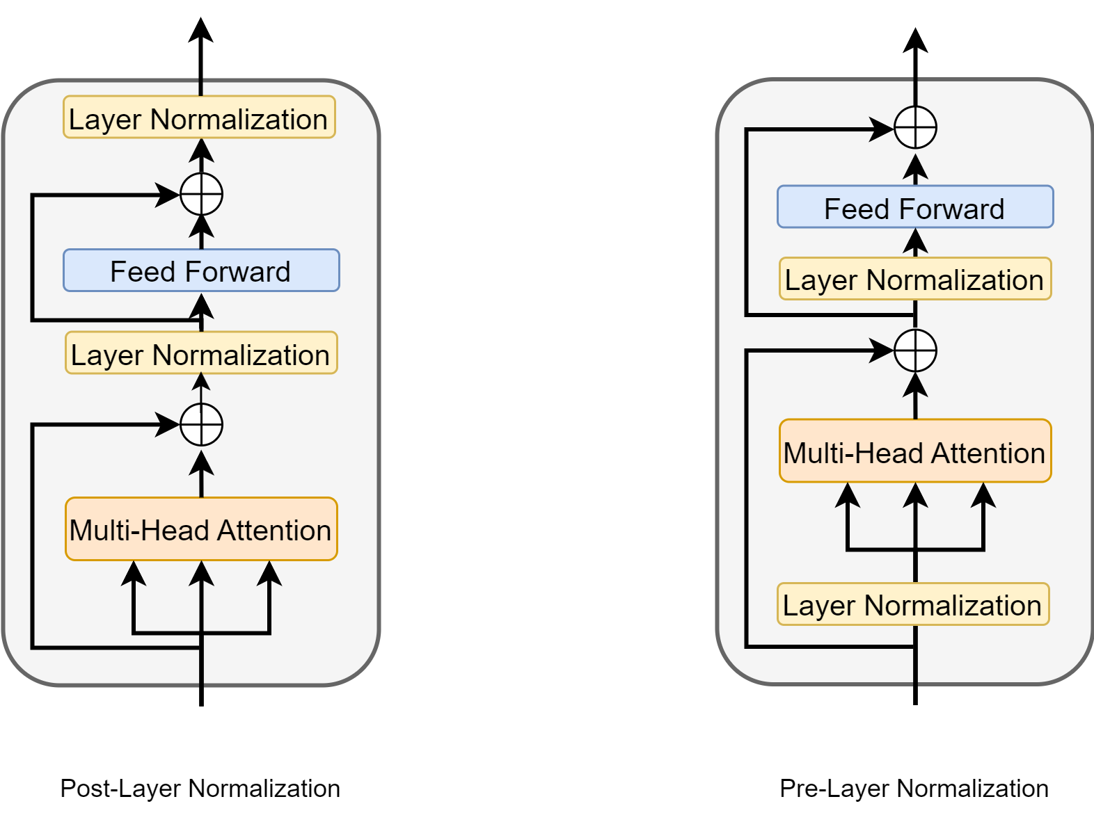
The Pre-LN architecture has become the standard for most modern LLMs (starting from GPT-2) because it keeps the gradient flow along the residual path "clean" and ensures that the inputs to each sub-layer are always well-behaved, preventing the exploding gradient problem in very deep models.

This article provides an excellent, detailed comparison.

Integrating LayerNorm into a Transformer Block

Now let's put it all together in code, using PyTorch's built-in nn.LayerNorm and the Pre-LN architecture. We also need to add the residual connections, which are simple additions.

Here's what the forward pass of a complete Transformer Block looks like using the Pre-LN architecture you just saw. This connects all the pieces we've learned in this module so far.

class Block(nn.Module):
    def __init__(self, n_embd, n_head):
        # n_embd: embedding dimension, n_head: the number of attention heads
        super().__init__()
        head_size = n_embd // n_head
        self.sa = MultiHeadAttention(n_head, head_size) # From a previous lesson
        self.ffwd = FeedForward(n_embd)              # From the last lesson
        self.ln1 = nn.LayerNorm(n_embd)
        self.ln2 = nn.LayerNorm(n_embd)

    def forward(self, x):
        # "Add & Norm" for Self-Attention
        # Residual connection adds the input 'x' to the output of the sub-layer
        x = x + self.sa(self.ln1(x))
        
        # "Add & Norm" for Feed-Forward Network
        x = x + self.ffwd(self.ln2(x))
        return x

Conclusion

You have now mastered one of the most critical and deceptively simple components of the Transformer. While attention and FFNs do the heavy computational lifting, Layer Normalization is the indispensable facilitator that ensures the entire deep network can be trained stably and efficiently.

Key Takeaways:

• Purpose: LayerNorm stabilizes training by normalizing the activations within each layer, preventing internal covariate shift and issues like exploding gradients.
• Mechanism: It normalizes across the feature dimension for each token independently, making it ideal for sequence data. It uses learnable gamma and beta parameters to retain expressive power.
• Placement is Key: The Pre-LN architecture (x + Sublayer(LayerNorm(x))) is the modern standard due to its superior training stability compared to the original Post-LN architecture.
• "Add & Norm": LayerNorm, combined with the residual connection, forms the "Add & Norm" blocks that wrap the self-attention and FFN sub-layers, creating a robust and trainable Transformer block.

What's Next?

We have now assembled all the fundamental components of a single Transformer block: multi-head attention, the position-wise FFN, positional encodings, residual connections, and layer normalization. In our next lesson, we will put everything together to trace the data flow through a full encoder and decoder block, showing how these pieces interact to process sequences and generate outputs. This will complete our foundational understanding of the Transformer's core mechanics.