Stateful Model Partitioning

The Partition-Transform-Merge Pattern

At a high level, handling state in a functional deep learning library follows a consistent pattern: you separate the static parts of your model (the parameters) from the dynamic parts (the state). You apply your core logic (the forward pass and gradient calculation) and generate an updated state. Finally, you merge the updated state back for the next iteration.

This abstract flow can be visualized as follows:

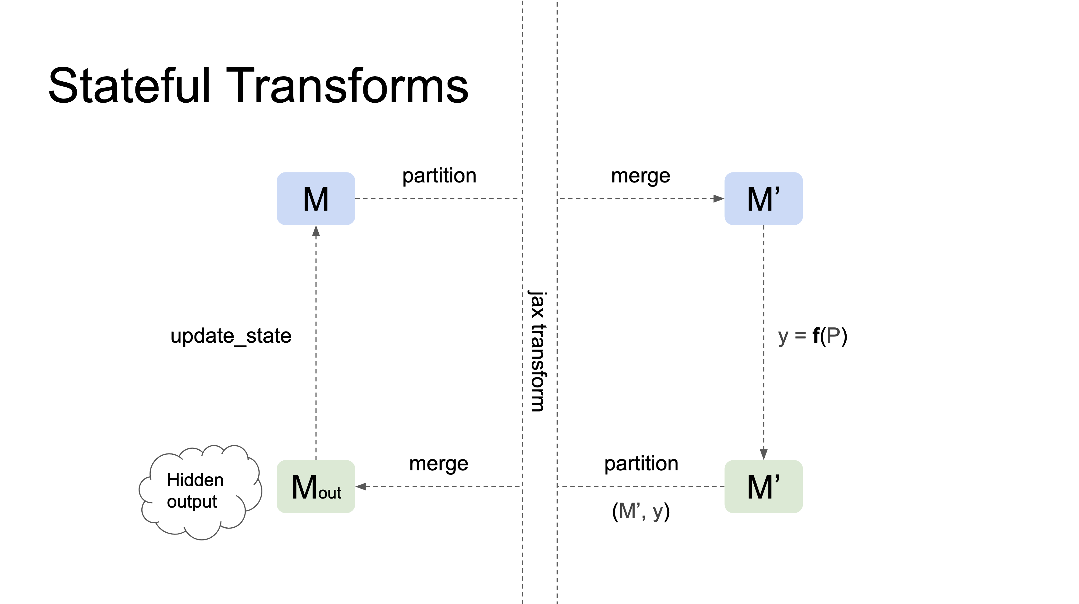
In this diagram, M represents the combined model and its state. It gets partitioned, transformed by a pure JAX function (y = f(P)), and the results are used to construct the output M_out. Our goal today is to understand how Equinox implements this pattern.

The Challenge of Evolving State

A layer like BatchNorm normalizes its inputs using the mean and variance of the current mini-batch during training. Crucially, it also maintains an exponential moving average of the mean and variance encountered across all training batches. These running statistics are what's used during inference to normalize a single example.

In an object-oriented framework, this is simple:
self.running_mean = momentum * self.running_mean + (1 - momentum) * batch_mean

This is a side effect—a mutation of the object's internal state. Since JAX transformations like jit require pure functions (no side effects), this approach is not viable.

The functional solution, consistent with our previous lesson, is to make the state explicit. A stateful function must:

1. Accept the current state as an input.
2. Return the new, updated state as an output.

So, a stateful layer's call signature becomes y, new_state = layer(x, old_state).

Equinox's Approach: make_with_state

Equinox provides a clean and powerful abstraction for this pattern. Instead of you manually tracking which parts of your model are parameters and which are state, Equinox offers a helper to do it for you.

The central tool is eqx.nn.make_with_state. When you define a model class containing stateful layers (like eqx.nn.BatchNorm), you don't instantiate it directly. Instead, you wrap the constructor with this function.

model, state = eqx.nn.make_with_state(MyModel)(key)

This call does two things:

1. It calls MyModel(key) to create a temporary, monolithic pytree containing both parameters and the initial values for the stateful components.
2. It then partitions this tree into two separate pytrees:
   • model: Contains the model structure and all trainable parameters (like Linear weights). All stateful components are replaced by placeholders.
   • state: A special eqx.nn.State object that holds the initial values for the BatchNorm running statistics.

Let's examine a complete example from the Equinox documentation.

As you can see, every layer that is stateful (in this case, BatchNorm and SpectralNorm) is called in a way that passes the state object through it, receiving an updated version. The non-stateful layers (Linear, relu) are used as normal.

Under the Hood: State and StateIndex

Given your background in mathematics and computing, you'll likely appreciate understanding the mechanism behind this. The state object isn't magical; it's a well-defined data structure.

The API documentation for stateful operations provides insight.

To summarize the mechanism:

• Every stateful layer instance (e.g., self.norm1 in the previous example) contains an eqx.nn.StateIndex. This is a unique, hashable identifier for that specific piece of state.
• The state object that is passed around is an instance of eqx.nn.State, which acts like a dictionary mapping each StateIndex to its corresponding value (e.g., the running mean and variance arrays).
• When a layer needs to update its state, it first retrieves its current value with current_val = state.get(self.index), computes the new value, and then creates a new state object with new_state = state.set(self.index, new_val).
• This immutability is key. state.set does not modify the state object in-place; it returns a new one. This preserves functional purity.

Integrating State into the Training Step

Now, let's connect this back to our jit-compiled training step. We need to modify our functions to handle this new state object.

1. The Loss Function: The function that computes the loss must now accept the state as an argument and return the updated state as an auxiliary output. Its signature will be loss_fn(model, state, x, y) and it will return (loss, new_state).

2. Gradients with has_aux: jax.grad (and its Equinox wrapper) has a has_aux argument precisely for this scenario. When has_aux=True, JAX knows the function returns a tuple (primary_output, auxiliary_data). It will compute gradients with respect to the primary_output (the loss) and simply pass the auxiliary_data (the new state) through as a return value.

3. The Step Function: Our make_step function now takes state as an input and returns the updated state as an output.

The following resource shows how these pieces fit together.

The full workflow is:
grads, new_state = eqx.filter_grad(compute_loss, has_aux=True)(model, old_state, ...)
Then you use grads to update the model, and you pass new_state to the next training step. The training loop becomes a simple loop that carries the model, state, and opt_state from one iteration to the next.

Handling Inference

During inference, two things change:

1. We want to use the final, trained running statistics for BatchNorm, not the statistics of the (potentially single-item) inference batch.
2. We no longer need to update the state.

Equinox provides helpers for this as well.

The process is straightforward:

1. inference_model = eqx.nn.inference_mode(model): This creates a copy of the model where layers like BatchNorm and Dropout are permanently switched to inference mode.
2. inference_model = eqx.Partial(inference_model, state=state): eqx.Partial is a utility that "bakes" arguments into a function. Here, we are creating a new callable object where the state argument of the model's __call__ method is pre-filled with our final, trained state.

The resulting inference_model can be called simply as y, _ = inference_model(x). You no longer need to pass the state in, making for a much cleaner API at evaluation time.

Conclusion

Today we have closed the loop on how to build and train sophisticated models in JAX and Equinox. By embracing the functional pattern of explicit state management, we can handle complex components like BatchNorm within a pure, jit-compilable framework.

Key Takeaways:

• Evolving state, such as BatchNorm running statistics, must be handled explicitly in pure functional code.
• The core pattern is to partition the model into trainable parameters and evolving state. eqx.nn.make_with_state is the main tool for this.
• The state object is threaded through the model's forward pass and the training step, which accepts the old state as input and returns the new state as output.
• eqx.filter_grad(..., has_aux=True) is used to differentiate a loss function that returns both a scalar loss and an updated state object.
• For inference, eqx.nn.inference_mode switches the model to evaluation behavior, and eqx.Partial can be used to bake the final trained state into the model for a simpler API.

You now possess the complete toolkit for defining model structure and behavior. In the next module, we will turn our attention to the training process itself, diving into the Optax library to construct powerful optimizers and build our final, production-ready training and evaluation loops.