Efficient Loops with `jax.lax.scan`

1. The Trouble with Python for Loops

Just as a standard Python if statement can cause issues with jit, so can a standard for loop. The JAX tracer attempts to handle for loops by "unrolling" them. If a loop runs a fixed number of times, say 10, the tracer will inline the body of the loop 10 times into the jaxpr.

@jax.jit
def f(x):



  # This loop will be unrolled by the JAX tracer
  for _ in range(10):
    x = jnp.sin(x)
  return x

While this works, it's often inefficient. Unrolling leads to larger compiled code and longer compile times. More importantly, if the number of iterations depends on a traced value, the tracer cannot determine the loop bounds and will fail, much like the if statement we saw before.

The JAX solution is to provide a primitive that represents the entire loop as a single, compilable operation: jax.lax.scan. This allows XLA to compile the loop body once and apply it iteratively, and in many cases, to apply powerful parallelization strategies that are impossible with an unrolled Python loop.

2. The Anatomy of jax.lax.scan

At its core, jax.lax.scan is designed for computations that iterate over a sequence of data while carrying along a state. Its signature is jax.lax.scan(f, init, xs).

The key is the function f, which must have the signature: (carry, x) -> (carry, y). Let's break this down:

• carry: This is the state of the loop. It is passed from one iteration to the next, allowing you to maintain and update information over time. Think of it as the hidden state in an RNN.
• x: This is a single "slice" from the input sequence xs. At each step, scan feeds one element from xs into your function.
• The function f returns a tuple (new_carry, y).
  • new_carry: The updated state that will be passed as the carry to the next iteration.
  • y: A per-iteration output. scan collects all the y values from each step and stacks them into a single output array.

The main jax.lax.scan call itself returns a tuple (final_carry, ys).

• final_carry: The final value of the carry state after the last iteration.
• ys: The stacked array of all the per-iteration y outputs.

This structure is best understood with a visual example. The following diagram illustrates the components of scan using a simple cumulative sum calculation.

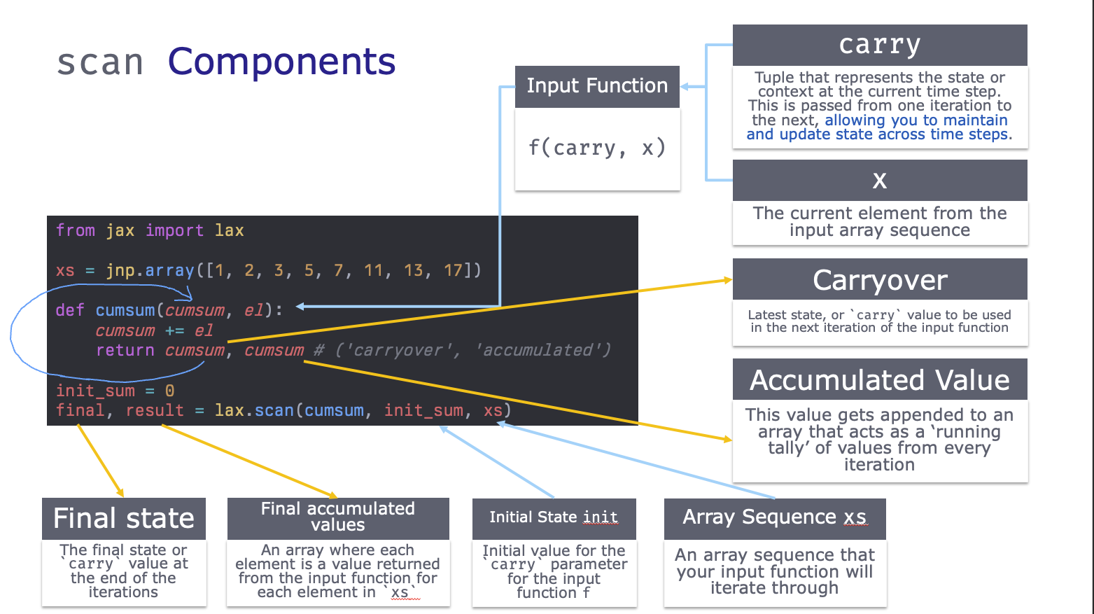
Let's trace the cumsum example from the image:

• init_sum = 0 is our initial carry.
• xs = jnp.array([1, 2, 3, ...]) is our input sequence.
• Iteration 1: f is called with carry=0 and x=1. It calculates cumsum = 0 + 1 = 1. It returns (1, 1).
  • The new carry for the next iteration is 1.
  • The first accumulated output y is 1.
• Iteration 2: f is called with carry=1 and x=2. It calculates cumsum = 1 + 2 = 3. It returns (3, 3).
  • The new carry is 3.
  • The second accumulated output y is 3.
• ...and so on.

The final result of lax.scan will be (final_sum, [1, 3, 6, 11, ...]), where final_sum is the total sum of all elements, and the second element is the array of cumulative sums at each step.

3. Recurrent Patterns, Differentiation, and Vectorization

The true power of lax.scan becomes apparent when implementing recurrent models, a task central to your work in deep learning. The carry state maps perfectly to the concept of a hidden state in an RNN.

This is where scan's composability with grad and vmap shines. The following resource provides an excellent, compact explanation and a code example for implementing a simple RNN, and then vectorizing it across a batch.

Let's consolidate what you've just read.

Differentiating Through Recurrence

The simple_rnn_step function you saw is the core of the recurrence:
new_hidden = jnp.tanh(W * x_t + U * prev_hidden + b)

When you wrap this step function in lax.scan, you are defining the entire forward pass of the RNN over a sequence.
final_hidden, outputs = lax.scan(simple_rnn_step, initial_hidden, inputs)

The remarkable part is what happens when you apply jax.grad.
grad_run_rnn = jax.grad(run_rnn, argnums=0)

JAX traces the computation through the unrolled steps of the scan and applies the chain rule automatically. You get the gradient of the final loss with respect to the initial hidden state (or any other parameter) without ever manually implementing BPTT. The scan primitive provides the necessary structure for JAX to handle this complex dependency tracking.

Vectorizing Recurrence for Batching

In practice, you never process a single sequence at a time. The combination vmap(scan(...)) is the standard JAX idiom for a batched RNN forward pass.

batched_run_rnn = jax.vmap(run_rnn, in_axes=(0, 0))

Here, in_axes=(0, 0) tells vmap that both the initial hidden state and the input sequence are batched along their first axis. JAX is smart enough to push the vmap transformation inside the scan, so that each of the batch_size sequences is processed by its own independent recurrent loop, all in parallel on the accelerator.

This composition—jit(grad(vmap(scan(...))))—is a powerful pattern for building and training sequence models in JAX.

4. scan vs. fori_loop

JAX provides another, simpler loop primitive: jax.lax.fori_loop(lower, upper, body_fun, init_val). This is closer to a standard for i in range(...) loop.

• It iterates a fixed number of times (upper - lower).
• The body_fun has the signature (i, val) -> val, where i is the loop index and val is the loop-carried state.
• It does not scan over an input array xs.
• It does not accumulate per-iteration outputs ys. It only returns the final value of the state.

You should use fori_loop when you simply need to apply a function a fixed number of times, like in an optimization loop. Use scan when you need to iterate over a data sequence, accumulate outputs, or both—which is the common case for neural network layers (e.g., stacking Transformer blocks, which we'll see in a future module).

Conclusion

You now have the primary tool for iteration in your JAX arsenal. jax.lax.scan is not just a jit-compatible for loop; it is a high-performance, differentiable primitive for expressing sequential and recurrent computations. Mastering its (carry, x) -> (carry, y) pattern is key to implementing sophisticated models.

Key Takeaways:

• Python for loops are often inefficient or incompatible with jit because they are unrolled.
• jax.lax.scan provides a compilable, parallelizable primitive for iteration.
• The core of scan is a function with the signature (carry, x) -> (carry, y) that updates a state (carry) while iterating over an input sequence (xs).
• scan composes seamlessly with grad to enable automatic differentiation through recurrence (BPTT).
• The combination vmap(scan(...)) is the canonical pattern for processing batches of sequences.
• jax.lax.fori_loop is a simpler alternative for fixed-iteration loops that don't need to process an input sequence or collect intermediate results.

In our examples, the carry and xs have been simple JAX arrays. However, in real models, the state you carry can be much more complex—a dictionary of parameters, a tuple of hidden and cell states for an LSTM, etc. JAX handles these complex, nested data structures through a system called pytrees. In our next lesson, we will dive into what pytrees are and how to manipulate them, unlocking the ability to build and train full-scale neural networks.