Welcome back! In our previous lessons, we've been dissecting the mechanics of automatic differentiation in JAX. We explored custom_vjp to rewrite the backward pass and stop_gradient to prune it for modeling purposes. Today, we'll examine our final AD-related topic in this module: a technique that modifies the backward pass not for algorithmic correctness, but for computational performance.
This lesson is about gradient checkpointing, a crucial technique for training very large neural networks. In JAX, this is often called rematerialization and implemented via jax.checkpoint or jax.remat. You'll learn how it allows you to trade a bit of extra computation for a significant reduction in memory usage, enabling you to train models that would otherwise be too large to fit on your accelerator. This is a vital tool, especially as we look ahead to implementing large-scale models like Transformers.
1. The Memory Cost of Reverse-Mode Autodiff
To understand why gradient checkpointing is necessary, we must first revisit the mechanics of reverse-mode automatic differentiation, the algorithm that powers backpropagation in modern deep learning frameworks.
As you know, reverse-mode AD is a two-stage process:
- Forward Pass: The function is executed, and the value of each intermediate operation (the activations in a neural network) and the structure of the computational graph are stored in memory.
- Backward Pass: Gradients are propagated backward from the output, using the stored activations and the chain rule to compute the derivative of the output with respect to each parameter.
The need to store all intermediate activations from the forward pass is the critical point. For a deep network with many layers, the memory required to hold these activations can be enormous, often exceeding the available RAM on a GPU or TPU. This can severely limit the maximum depth of your model or the batch size you can use during training.
To refresh your memory on this, let's watch a brief segment from a video on automatic differentiation.
What is Automatic Differentiation?
This video from Ari Seff provides a clear overview of different AD methods. We'll focus on the part explaining reverse-mode AD and its memory requirements.
Please watch the segment on reverse mode autodiff, which explains the two-pass process. Then, pay close attention to the short follow-up that explicitly mentions its memory intensiveness and introduces the idea of re-materialization.
The key takeaway is that the efficiency of reverse-mode AD (one pass for the full gradient) comes at the cost of high memory usage. When this memory cost becomes prohibitive, we need a way to reduce it.
2. The Mechanism of Gradient Checkpointing
Gradient checkpointing, or rematerialization, offers a direct solution to this memory problem. The core idea is simple yet powerful: instead of storing all intermediate activations during the forward pass, we strategically discard most of them and recompute them on-the-fly during the backward pass as they are needed.
This involves selecting certain layers as "checkpoints" and only storing their outputs.
Here's how it works:
- Forward Pass: We execute the full forward pass as usual to get the final output. However, we only save the activations at designated checkpoint locations. All other intermediate activations are discarded.
- Backward Pass: As the gradient signal propagates backward, whenever it needs an activation that was discarded, the system finds the nearest preceding checkpoint. It then performs a localized forward pass from that checkpoint up to the required point to "rematerialize" the needed activation.
This creates a direct trade-off:
- Memory ↓: We save a significant amount of memory by not storing the bulk of the activations.
- Compute ↑: We incur additional computational cost because parts of the forward pass are re-executed during the backward pass.
The following diagram illustrates this trade-off visually.
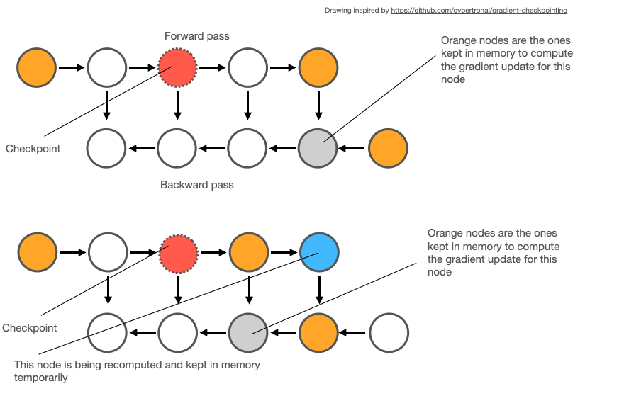
In the top diagram, every activation from the forward pass is stored to be used in the backward pass. In the bottom diagram, we only checkpoint the output of certain layers (the orange nodes). During the backward pass, to compute the gradient at the gray node, the system needs the activation of the preceding white node. Since it wasn't stored, it's recomputed by running a forward pass from the red checkpointed node.
3. Gradient Checkpointing in JAX
In JAX, gradient checkpointing is implemented with jax.checkpoint (aliased as jax.remat). While you can wrap any function with it, it's most powerfully used in combination with jax.lax.scan for implementing sequential models. As you're interested in implementing Transformers, this "scan-over-layers" pattern is something you'll become very familiar with.
The documentation for the Haliax library (a high-level wrapper around JAX) provides an exceptionally clear explanation of the different checkpointing policies, which map directly to JAX's underlying capabilities.
This document explains gradient checkpointing in the context of scan, which is the idiomatic way to handle stacks of layers in JAX. The principles and policies described here are fundamental to JAX itself.
First, read the brief introduction in Gradient Checkpointing / Rematerialization. Next, review the TL;DR Guidance and Simple Checkpointing sections. This introduces the most common policy, remat=True. Then, read the section on Nested Scan. This explains the remat="nested" policy and the O(sqrt(N)) memory trade-off, which is a classic optimization. Finally, study the table in the section on Memory and Computation Tradeoffs. This table provides a quantitative summary of the costs associated with different policies.
Let's summarize the key policies and their trade-offs, using the notation from the article where N is the number of layers:
Policy (remat=...) |
Memory Usage | Computation Cost | Description |
|---|---|---|---|
False |
No Checkpointing: Store all activations. Maximum memory, minimum compute. | ||
True (Simple) |
Standard Checkpointing: Store layer inputs/outputs ("carries"), recompute layer internals. Good balance. | ||
"nested" |
Nested Checkpointing: Checkpoints every layers. Drastically cuts memory for a bit more compute. |
The computational costs are approximate (e.g., a forward pass + backward pass is , a recomputation adds another partial forward pass). The key insight is the asymptotic behavior. With remat="nested", you can train a model with 10,000 layers using roughly the same activation memory as a model with 100 layers, at the cost of about 20-25% more FLOPs. For large models, this is an excellent trade.
Fine-Grained Control
JAX also provides more advanced checkpointing policies for fine-grained control, which the Haliax document also touches upon. For example, you can specify exactly which intermediate values within a function to save, or even offload checkpoints from accelerator memory to host (CPU) RAM, further reducing the on-device memory footprint at the cost of slower data transfers. These advanced options give you precise control over the memory-compute trade-off.
Conclusion
Today, we've unpacked gradient checkpointing (remat), a performance optimization technique that is indispensable for training large-scale deep learning models. You've learned that it's a direct response to the high memory demands of reverse-mode autodiff.
Key Takeaways:
- The Problem: Reverse-mode autodiff stores all intermediate activations from the forward pass, leading to high memory consumption in deep networks.
- The Solution: Gradient checkpointing saves memory by discarding most activations and recomputing them during the backward pass.
- The Trade-off: It trades increased computational cost for significantly reduced memory usage.
- JAX Implementation:
jax.checkpoint(orjax.remat) is the primary tool, often used withjax.lax.scan. Policies likeremat=Trueandremat="nested"offer different points on the memory-compute spectrum, with the latter providing anO(sqrt(N))memory footprint for activations.
This lesson concludes our deep dive into the mechanics of automatic differentiation in JAX. You now have a solid understanding of not only how to compute gradients, but also how to manipulate and optimize the process for both modeling and performance goals.
In our next module, we will move up a level of abstraction and begin building neural networks using Equinox. You will see how Equinox leverages JAX's functional nature and its pytree system to provide a powerful and intuitive way to define models, and how the transformations we've studied (jit, grad, vmap, and remat) integrate seamlessly into the model development workflow.