Logistic Regression: From Binary Classification to Probabilistic Modeling

From Linear Models to Probabilities

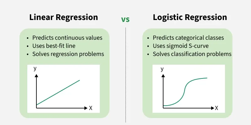
In our last lesson, we focused on regression models that predict continuous values. The simplest of these is a linear model, which computes a weighted sum of the input features:

$z={\mathbf{w}}^T\mathbf{x}+b$

This output, $z$, can be any real number from $-\infty$ to $+\infty$. This is fine for regression, but for binary classification, we need to predict a class (e.g., 0 or 1). A more powerful approach is to predict the probability that an input $\mathbf{x}$ belongs to the positive class (class 1). A probability, by definition, must be constrained to the range [0, 1].

So, how can we adapt our linear model to produce a valid probability? We need a function that takes any real number $z$ and "squashes" it into the (0, 1) interval. This is where the sigmoid function comes in.

The Sigmoid Function

The sigmoid function, also called the logistic function, is defined as:

$\sigma (z)=\frac{1}{1+e^{-z}}$

It has a characteristic S-shape and maps any real-valued input $z$ to an output between 0 and 1.

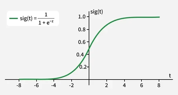
By feeding the output of our linear model into the sigmoid function, we create the core of the logistic regression model. We can now interpret the output as the estimated probability of the positive class:

$\hat{y}=P(y=1|\mathbf{x};\mathbf{w},b)=\sigma ({\mathbf{w}}^T\mathbf{x}+b)$

This equation represents the probabilistic heart of logistic regression. It explicitly models the probability of a positive outcome given the input features $\mathbf{x}$ and the model parameters $\mathbf{w}$ and $b$.

The article "Mastering Logistic Regression" provides an excellent description of this model structure, framing it in terms of "log-odds." The log-odds, or logit, is the inverse of the sigmoid function, and understanding this relationship gives a deeper insight into why logistic regression is considered a linear classifier.

The Cost Function for Logistic Regression

Now that we have a model that predicts probabilities, how do we train it? We need to find the parameters $\mathbf{w}$ and $b$ that make our predicted probabilities $\hat{y}$ as close as possible to the true labels $y$ (which are either 0 or 1).

This should sound familiar. In the previous lesson, we established that for a probabilistic classification model assuming a Bernoulli distribution for the outcomes, the appropriate loss function derived from Maximum Likelihood Estimation is Binary Cross-Entropy (BCE), also known as Log Loss.

For a single training example, the BCE loss is:

When we substitute our logistic regression model for $\hat{y}$, we get the loss function we need to minimize to train our model. The average of this loss over all training examples gives us our total cost function $J(\mathbf{w},b)$.

The following reading section shows this exact derivation, connecting the principle of Maximum Likelihood Estimation directly to the Log Loss function used in logistic regression.

For an alternative and more detailed walkthrough of this derivation, the following video explains it step-by-step.

Implementing Logistic Regression from Scratch

We now have all the conceptual pieces:

1. Model: $\hat{y}=\sigma ({\mathbf{w}}^T\mathbf{x}+b)$
2. Cost Function: Average Binary Cross-Entropy, $J(\mathbf{w},b)$
3. Goal: Find $\mathbf{w}$ and $b$ that minimize $J(\mathbf{w},b)$.

The algorithm we'll use to minimize the cost function is Gradient Descent. We will dive deep into the calculus and derivation of gradient descent in our next lesson. For today, we will focus on the implementation, using the final gradient formulas.

The core idea of gradient descent is to iteratively update the parameters in the direction opposite to the gradient of the cost function. The update rules are:
$\mathbf{w}:=\mathbf{w}-\alpha \frac{\partial J}{\partial \mathbf{w}}$
$b:=b-\alpha \frac{\partial J}{\partial b}$
where $\alpha$ is the learning rate.

The partial derivatives of the cost function $J$ with respect to the parameters turn out to have a surprisingly simple form:
$\frac{\partial J}{\partial \mathbf{w}}=\frac{1}{m}{\mathbf{X}}^T(\hat{\mathbf{y}}-\mathbf{y})$
$\frac{\partial J}{\partial b}=\frac{1}{m}{\sum }_{i=1}^m({\hat{y}}^{(i)}-y^{(i)})$

Here, $m$ is the number of training examples, $\mathbf{X}$ is the feature matrix, and $\hat{\mathbf{y}}$ and $\mathbf{y}$ are vectors of predicted probabilities and true labels, respectively.

Let's now see how to translate these mathematical ideas into a working Python implementation. We will use the "Mastering Logistic Regression" article as a guide.

To solidify this, here is a consolidated implementation structured as a Python class. This is a common and practical way to organize a model's logic.

import numpy as np

class MyLogisticRegression:
    """
    A simple implementation of Logistic Regression from scratch.
    """
    def __init__(self, learning_rate=0.01, n_iterations=1000):
        self.learning_rate = learning_rate
        self.n_iterations = n_iterations
        self.weights = None
        self.bias = None

    def _sigmoid(self, z):
        return 1 / (1 + np.exp(-z))

    def fit(self, X, y):



        # 1. Initialize parameters
        n_samples, n_features = X.shape
        self.weights = np.zeros(n_features)
        self.bias = 0




        # 2. Gradient Descent
        for _ in range(self.n_iterations):



            # Calculate linear model and apply sigmoid
            linear_model = np.dot(X, self.weights) + self.bias
            y_predicted = self._sigmoid(linear_model)




            # Calculate gradients
            dw = (1 / n_samples) * np.dot(X.T, (y_predicted - y))
            db = (1 / n_samples) * np.sum(y_predicted - y)




            # Update parameters
            self.weights -= self.learning_rate * dw
            self.bias -= self.learning_rate * db

    def predict_proba(self, X):
        linear_model = np.dot(X, self.weights) + self.bias
        return self._sigmoid(linear_model)

    def predict(self, X, threshold=0.5):
        probabilities = self.predict_proba(X)
        return [1 if i > threshold else 0 for i in probabilities]




# Example usage (you can try this with any binary classification dataset from scikit-learn)
# from sklearn.model_selection import train_test_split
# from sklearn.datasets import make_classification
# X, y = make_classification(n_samples=100, n_features=2, n_redundant=0, n_informative=2, random_state=1, n_clusters_per_class=1)
# X_train, X_test, y_train, y_test = train_test_split(X, y, test_size=0.2, random_state=123)




# model = MyLogisticRegression(learning_rate=0.1, n_iterations=1000)
# model.fit(X_train, y_train)
# predictions = model.predict(X_test)
# accuracy = np.mean(predictions == y_test)
# print(f"Accuracy: {accuracy:.2f}")

Spend a few moments studying this class. Notice how the fit method encapsulates the entire training loop, and the predict method uses the learned weights and bias to make new classifications.

Conclusion

In this lesson, we have constructed our first machine learning classifier from the ground up. You have seen how logistic regression seamlessly combines a linear model with a sigmoid function to produce probabilities, and how it is trained by minimizing a cost function (Binary Cross-Entropy) that is directly motivated by the principle of maximum likelihood.

Key takeaways from today's lesson:

• Logistic Regression is a probabilistic linear classifier for binary tasks.
• It models the probability of the positive class using a linear combination of features passed through the sigmoid function.
• The model is trained by minimizing the Binary Cross-Entropy (or Log Loss) function, which is equivalent to maximizing the likelihood of the training data under a Bernoulli distribution assumption.
• The implementation involves an iterative optimization process, Gradient Descent, which uses the gradients of the cost function to update the model's parameters.

We have used the gradient formulas to build our fit method. In our next lesson, we will put on our calculus hats and formally derive these gradient formulas. This will give you a complete understanding of Gradient Descent, the workhorse optimization algorithm for most of machine learning.