Optimizing Inference Throughput with Batching Strategies

Hello! Welcome to the fourth lesson in our module on Model Optimization and Deployment.

In our last lesson, you learned how to systematically compare different model acceleration techniques, weighing the speed (NFE) against the quality (FID). We saw that methods like distillation can drastically reduce the number of steps for a single image generation. Now, we'll shift our focus from optimizing a single inference to optimizing a service that handles many requests, which is the reality of a production environment.

Today's learning outcome is to implement and evaluate batching strategies to maximize inference throughput. As a lead ML engineer, you know that serving a model isn't just about single-request speed; it's about efficiently handling concurrent users and maximizing the utilization of expensive GPU hardware.

We will explore:

The fundamental trade-off between throughput and latency in inference serving.
An overview of common batching strategies: static, dynamic, and continuous batching.
How to configure models and servers like Triton to support these strategies.
The unique advantages of continuous batching for iterative diffusion models.
Methods for benchmarking and evaluating the performance of your chosen strategy.

1. The Core Trade-Off: Throughput vs. Latency

When deploying a model, we often care about two key performance indicators:

Latency: The time it takes to process a single request from start to finish. Lower is better. For a diffusion model, this is the wall-clock time to generate one image.
Throughput: The total number of requests the system can handle per unit of time (e.g., images per second). Higher is better.

GPUs excel at parallel computation. Running a batch of 8 inputs through a U-Net is significantly faster than running 8 individual inputs sequentially. This is the core principle of batching. However, it introduces a trade-off: to create a batch, the first request might have to wait for other requests to arrive, increasing its individual latency. Your goal as an engineer is to find the sweet spot that meets your service-level objectives (SLOs).

The image below illustrates different ways to handle incoming requests, which we will explore in this lesson.

Batching Strategies for LLM Inference — This image visualizes three different approaches to handling inference requests. "Individual Requests" processes one at a time. "Dynamic Batching" groups several requests together. "Continuous Batching" shows a more fluid packing of requests, hinting at better resource utilization.

2. Static Batching: The Simple Approach

The most basic strategy is static batching. You define a fixed batch size, say N=8, and the server waits until it has collected 8 requests before sending them to the GPU for processing.

Accelerate Serving Stable Diffusion by Optimizing the ...

The article 'Accelerate Serving Stable Diffusion' from Lightning AI begins by describing this traditional approach and its significant drawbacks.

Read the section 'Traditional inference method'. It uses a great coffee shop analogy to explain the latency problem and highlights how this strategy can lead to underutilized servers.

Pros:

Simple to implement.

Cons:

High Latency: The first request in a batch experiences high latency as it waits for the batch to fill.
Poor Utilization: If requests arrive slowly, the GPU sits idle while the server waits. If a new request arrives just after a batch has been dispatched, it must wait for the next full batch.

Due to these significant drawbacks, static batching is rarely used in modern, high-performance serving systems.

3. Dynamic Batching with Triton and TensorRT

A major improvement is dynamic batching. Here, the server collects requests for a short period (a timeout) and then sends whatever it has collected (up to a maximum batch size) for processing. This balances the need to form batches with the need to keep latency low.

Many modern inference servers, like NVIDIA's Triton Inference Server, support this out of the box. However, to use it, your model must be optimized to accept a variable batch size. This is where TensorRT comes in.

First, let's understand what TensorRT does and why it's important for this process.

Inference Optimization with NVIDIA TensorRT

The video 'Inference Optimization with NVIDIA TensorRT' provides a concise overview of what TensorRT is and the optimizations it performs.

Watch the first section (0:52 - 5:44) to understand TensorRT's core purpose, including layer fusion and quantization. Then, watch the overview of the conversion process (5:44 - 9:05). Pay close attention to the parameters specified during conversion, such as 'desired batch size'. This is the key to enabling batching in the optimized model.

The key takeaway is that when you convert your model (e.g., the U-Net) to a TensorRT engine, you're not just making it faster; you're also defining its operational parameters, including the range of batch sizes it can handle.

The following guide provides a fantastic, practical walkthrough of this entire process for a Stable Diffusion model.

A Practical Guide to Deploying Diffusion Models with Triton and TensorRT

The article 'A Practical Guide to Deploying Diffusion Models with Triton and TensorRT' details the end-to-end process of preparing a model for high-performance serving.

Focus on these three key steps from the article: Step 1: Export Models to ONNX: Notice the dynamic_axes configuration. This is the first step to tell the model that the batch dimension is not fixed. Step 4: Optimize with TensorRT: Look at the trtexec command. The --minShapes, --optShapes, and --maxShapes flags are where you explicitly define the range of batch sizes your engine will support (e.g., 1 to 4). Step 5: Configure Triton Models: Examine the config.pbtxt. Setting max_batch_size: 0 and using -1 in the input dims tells Triton that the model supports dynamic batching and that Triton should handle the request scheduling.

By following this process, you create a system where:

Your U-Net is compiled by TensorRT to be highly optimized for a specific range of batch sizes on your target GPU.
Triton Inference Server automatically intercepts incoming requests, batches them dynamically based on traffic, and sends them to the TensorRT engine for processing.

This is a powerful, industry-standard approach for serving many types of deep learning models, including the components of a diffusion pipeline (Text Encoder, U-Net, VAE).

4. Continuous Batching: The State-of-the-Art for Diffusion

While dynamic batching is a huge step up, we can do even better. Diffusion models have a unique iterative structure that we can exploit. A standard 20-step generation involves 20 separate forward passes of the U-Net.

Continuous batching (also known as iteration-level batching) takes advantage of this. Instead of waiting for whole generation requests to finish, it can add new requests into the batch at each denoising step.

Here's how it works:

An initial request arrives. The server starts its 20-step denoising process.
After, say, 5 steps, a new request arrives.
For step 6, the server forms a batch containing two items: the first request at denoising step 6, and the new request at denoising step 1.
The server passes this heterogeneous batch to the U-Net, ensuring the correct timestep is provided for each item in the batch.
When an item in the batch finishes its final step, it is removed and its result is returned to the user, while other items continue processing.

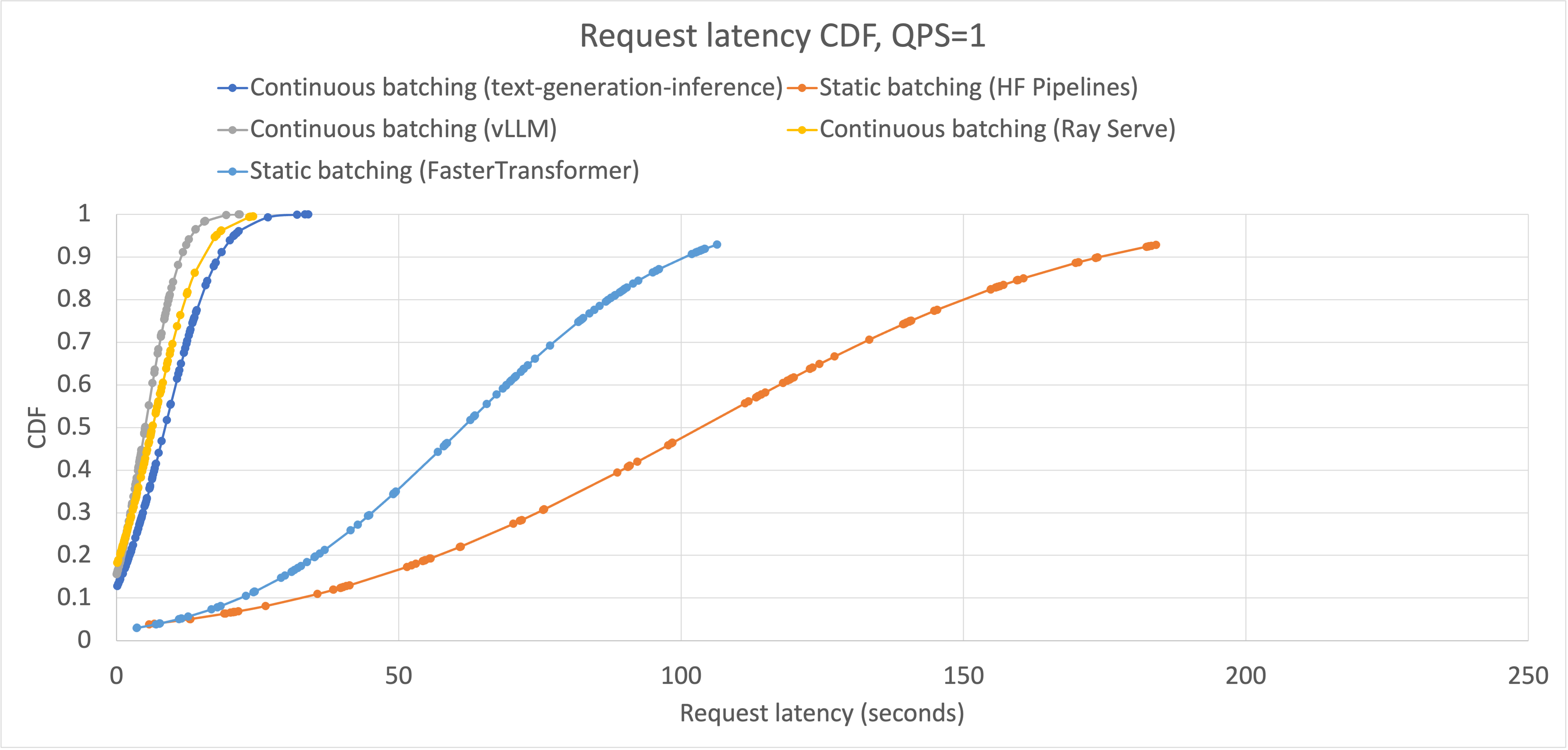
This strategy dramatically improves server utilization and reduces average request latency.

Accelerate Serving Stable Diffusion by Optimizing the ...

The same Lightning AI article we saw earlier introduces this novel approach and explains its implementation.

Read the sections 'Leveraging the diffusion process to accelerate inference' and the step-by-step breakdown that follows. Pay attention to the illustrations and logs, which clearly show how new requests join the batch mid-process. The pseudo-code using asyncio demonstrates the server-side logic required to manage the state of each request independently.

The performance gains from this approach are significant, as shown by benchmarking data comparing static and continuous batching strategies.

Request Latency CDF for Different Batching Strategies — This Cumulative Distribution Function (CDF) plot shows request latency for different batching strategies. Notice how the 'Continuous batching' lines are shifted to the left, indicating that they complete the vast majority of requests at a much lower latency compared to 'Static batching' methods.

Test your understanding!

You are designing a diffusion model serving system. You anticipate very high, continuous traffic. Your primary business goal is to serve as many users as possible with your existing hardware (maximize throughput), but you also have a Service Level Objective (SLO) that 95% of requests should have a latency under 2 seconds.

Which batching strategy would you choose and why? What are the key implementation challenges you would face?

Show answer

Strategy: Continuous batching is the ideal choice.

Reasoning:

Throughput: It maximizes GPU utilization by ensuring the GPU is almost always processing a full batch, directly addressing the goal of serving the most users.
Latency: By allowing new requests to start immediately without waiting for an entire generation cycle to complete, it dramatically reduces average and p95 latency, helping to meet the 2-second SLO. Static or even standard dynamic batching would likely lead to SLO violations under high load due to queuing delays.

Implementation Challenges:

State Management: The server logic is more complex. You need to track the current denoising step, latent state, and text conditioning for every single request currently in flight.
Heterogeneous Batches: The model's forward pass must be able to handle a batch where each item corresponds to a different timestep t. This means the timestep conditioning mechanism must be able to accept a batch of different t values, rather than a single scalar t.

5. Evaluating Batching Performance

To evaluate your chosen strategy, you need to conduct load testing. This involves simulating real-world traffic and measuring performance.

Key Metrics:

Throughput (Requests/Second): The primary measure of server capacity.
Latency Distribution (p50, p95, p99): Crucial for understanding the user experience. A low average latency (p50) is good, but a high p99 latency means some users are having a very slow experience.
GPU Utilization: A measure of how effectively you are using your hardware. Aim for consistently high utilization (e.g., >90%) under load.

Benchmarking Process:

Deploy your model using an inference server (like Triton) configured with your chosen batching strategy.
Use a load-testing tool (like Locust, as mentioned in the LINK article) to generate concurrent requests to your server endpoint.
Vary the load (e.g., number of concurrent users or queries per second) and record the throughput and latency metrics at each level.
Analyze the results to find the breaking point of your system and verify that you are meeting your performance SLOs.

The performance tables in the Triton guide (LINK, section "Performance Comparison") and the Lightning AI article (LINK, section "Benchmarking Serving Strategies") are excellent examples of the kind of output you would generate from such an evaluation.

Conclusion

You have now learned how to take an optimized model and deploy it for high-throughput inference, moving from single-sample speed to service-level performance.

Key Takeaways:

Batching is essential for maximizing GPU throughput, but it introduces a trade-off with request latency.
Static Batching is simple but inefficient.
Dynamic Batching, supported by tools like Triton, offers a robust and general-purpose solution by forming batches on-the-fly. This requires models to be compiled with tools like TensorRT to support variable batch sizes.
Continuous Batching is a state-of-the-art technique for diffusion models that leverages their iterative nature to achieve maximum throughput and minimum latency.
Systematic benchmarking with load-testing tools is critical to validate performance and ensure SLOs are met.

Next Lesson Preview:

Optimizing for throughput by increasing batch size often pushes your GPU's memory to its limits. What do you do when you run out of VRAM? In our next lesson, you will learn to profile and debug memory bottlenecks in diffusion training and inference pipelines, giving you the tools to manage one of the most common constraints in deep learning.