Latent Variable Propagation for Frame Consistency

From Pixel-Space to Latent-Space Conditioning

Last time, the core operation was essentially U-Net(concat(z_0^(n-1), z_t^n), t), where z_0^(n-1) is the final, fully denoised latent of the previous frame. This is a form of conditioning on a finished product.

Latent variable propagation (LVP) is about influencing the process of generation. The information from frame n-1 is used to structure the denoising steps of frame n. This creates a more fluid and deeply connected link between frames. The diagram below offers a high-level conceptual view of this feedback loop.

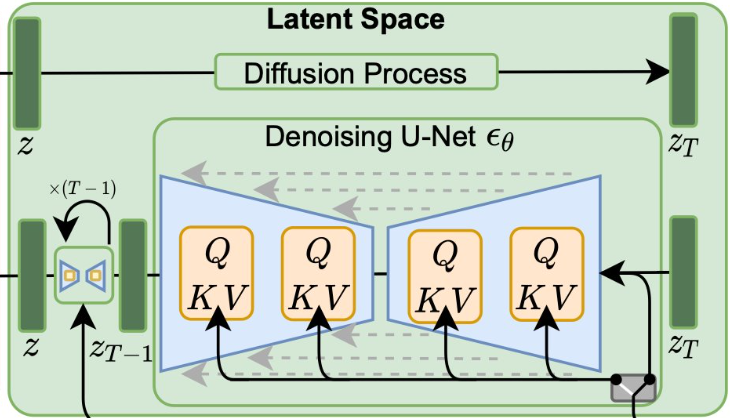
Let's now explore two concrete implementations of this concept.

Method 1: Previous Latent as a Noise Prior

Our first method comes from the paper "Glad: A Streaming Scene Generator," which proposes a frame-by-frame generation style with a dedicated Latent Variable Propagation (LVP) module.

The core idea is to treat the denoised latent features of the previous frame as the noise prior for the current frame. In a standard DDPM, the noise ε added to an image is sampled from a simple Gaussian distribution, N(0, I). In this LVP approach, the noise distribution is structured by the previous frame.

As you've read, the forward diffusion process for frame n is modified. Let's look at the key part of Equation (1):

In a standard DDPM, the covariance matrix of the noise is simply ${\beta }_t\mathbf{I}$. Here, it is replaced with ${\beta }_t\phi ({\mathbf{z}}_0^{n-1})$, where ${\mathbf{z}}_0^{n-1}$ is the fully denoised latent of the previous frame. The function $\phi$ is a normalization layer (like LayerNorm) to make the latent's statistics similar to that of noise.

Intuition: The model is no longer predicting unstructured Gaussian noise. It's trained to predict noise that is correlated with the structure of the previous frame. This implicitly guides the current frame to be a plausible continuation of the last one.

Implementation for Training and Inference

This theoretical change has direct consequences for your implementation, particularly in how you handle data during training and how you structure the inference loop.

From a practical engineering perspective, here's the breakdown:

• Training (Streaming Data Sampler): To ensure consistency between training and inference, you can't just pick random pairs of frames. You need to process video clips sequentially.

  1. For a given video clip, start with frame 1. The "previous frame" can be pure Gaussian noise.
  2. Train the model on frame 1 to predict the target noise. The model outputs a denoised latent ${\hat{\mathbf{z}}}_0^1$.
  3. Crucially, instead of discarding this, you use the ground-truth latent of frame 1, ${\mathbf{z}}_0^1$, as the noise prior for training on frame 2. You cache this latent.
  4. At iteration 2, you train on frame 2, using the cached ${\mathbf{z}}_0^1$ to structure the noise as per Eq. (1). You then use the ground-truth ${\mathbf{z}}_0^2$ as the prior for frame 3, and so on.
     This "streaming" approach ensures the model is trained in the same autoregressive manner it will be used in for inference.

• Inference: The inference loop directly mimics the training process.

  1. Generate frame n-1 and get its fully denoised latent ${\hat{\mathbf{z}}}_0^{n-1}$.
  2. To generate frame n, instead of starting the reverse diffusion process from pure random noise ${\mathbf{z}}_T^n\sim \mathcal{N}(0,I)$, you initialize the process using ${\hat{\mathbf{z}}}_0^{n-1}$ as the noise prior. The paper states this as $p({\mathbf{z}}_T^n)=p({\mathbf{z}}_0^{n-1})$, meaning the starting "noise" for frame n is simply the denoised latent from frame n-1.
  3. You then run the standard reverse diffusion process to generate ${\hat{\mathbf{z}}}_0^n$.
  4. Repeat for the desired number of frames.

This method provides a strong, direct link between frames by weaving the structure of one frame into the very noise distribution of the next.

Method 2: Consistent Context-Aware Inference

Our second method offers a different, equally powerful way to propagate latent information. It comes from the paper "ChronoDepth," which focuses on temporally consistent video depth estimation, but the mechanism is general-purpose.

The core idea is to use the previous frame's clean latent as a noiseless, fixed condition for a portion of the next generative clip, rather than using it to define the noise. This requires a unique training strategy to work.

This strategy is clever and has two key parts: a training modification and a corresponding inference procedure.

• Training Modification: The model must learn to denoise different frames that are at different noise levels within the same clip. Instead of sampling one noise level ${\omega }_t$ for the whole clip, you sample an independent noise level ${\omega }_i$ for each frame i in the clip. The U-Net's conditioning input for noise now becomes a per-frame variable. This prepares the model for the unusual inputs it will see during inference.

• Inference (Sliding Window with Overlap):

  1. Generate the first clip (e.g., frames 0-15) using the standard denoising process, starting from pure noise.
  2. To generate the next clip, which overlaps with the first (e.g., frames 8-23, with an overlap of 8 frames), you do the following for each denoising step t:
     • The overlapping part (frames 8-15): Initialize these frames with the final, clean latents ${\hat{\mathbf{z}}}_0^{8:15}$ from the previous generation. You do not add noise to them.
     • The new part (frames 16-23): Initialize these with standard noisy latents ${\mathbf{z}}_t^{16:23}$.
     • Concatenate and Denoise: The input to the U-Net at step t is a concatenation of the clean past and the noisy future: concat(z_0^(8:15), z_t^(16:23)).
     • Noise Level Conditioning: The model is told the noise level for the first part is effectively zero (or a very small constant ${\omega }_{\vartheta }$) and the noise level for the second part is ${\omega }_t$.
  3. The model's output is a denoised prediction for the entire clip, but you only use the new part ($16:23$) to update your latents for the next step. The clean part acts as a fixed anchor.

This method ensures the model's prediction for the new frames is perfectly consistent with the already-generated frames at every single step of the denoising process, virtually eliminating the flickering artifacts that can occur at clip boundaries.

# z_t.shape: (B, F, C, H, W)
# noise_levels.shape: (B, F)

# The preconditioning functions (cskip, cout, cin, cnoise) expect
# a noise level for each element in the batch. Here, our "elements"
# are individual frames. We need to reshape the inputs to treat
# frames as batch items.

B, F, C, H, W = z_t.shape

# Reshape latents and noise levels so frames are in the batch dimension
z_t_reshaped = z_t.view(B * F, C, H, W)
noise_levels_reshaped = noise_levels.view(B * F)

# Now, the standard preconditioning functions will work correctly
# as they receive a batch of size B*F.
c_skip = cskip_function(noise_levels_reshaped) # Shape: (B*F, 1)
c_out = cout_function(noise_levels_reshaped)   # Shape: (B*F, 1)
c_in = cin_function(noise_levels_reshaped)     # Shape: (B*F, 1)

# These need to be broadcast to match the reshaped latent tensor.
# For example, when applying c_in:
model_input = c_in.view(B * F, 1, 1, 1) * z_t_reshaped

# The noise embedding for the U-Net itself would also use the reshaped levels.
# c_noise_embedding = cnoise_function(noise_levels_reshaped) # Shape: (B*F, D)

# After the U-Net forward pass, the output would be reshaped back to
# (B, F, C, H, W) if needed.

Conclusion

In this lesson, we have moved beyond simple frame-concatenation and explored two sophisticated methods for latent variable propagation to ensure temporal consistency.

Key Takeaways:

• Latent Variable Propagation (LVP) creates a more deeply integrated temporal link than conditioning on the final output of the previous frame.
• The "Glad" LVP approach uses the previous denoised latent to create a structured noise prior, guiding the generation of the current frame. This is implemented with a sequential, "streaming" training and inference pipeline.
• The "ChronoDepth" Consistent Context-Aware approach uses the previous clean latents as a fixed, noiseless anchor in a sliding window. This requires a special training strategy where the model learns to handle per-frame noise levels.
• Both methods are powerful techniques for generating long, coherent videos by explicitly managing the flow of information between frames at the latent level.

Next Lesson Preview:

So far, our consistency mechanisms have been autoregressive, meaning each frame depends only on the one(s) that came before it. In the next lesson, we will explore a different paradigm: applying temporal attention for coherent video generation. This non-autoregressive approach allows every frame in a clip to attend to every other frame, enabling the model to capture complex, non-sequential relationships and generate all frames in parallel. This will be a key building block for more advanced video generation architectures.