Introduction to Neural Radiance Fields (NeRF)

1. The Core Idea: A Scene as a Continuous Function

At its heart, NeRF solves the problem of novel view synthesis: generating new images of a scene from arbitrary camera angles, given a sparse set of input images.

Instead of storing geometry explicitly (like in a voxel grid or mesh), NeRF represents a scene using a single, continuous function, typically a Multi-Layer Perceptron (MLP). The key idea is to "overfit" this small network to a single scene, encoding all the scene's information within the network's weights.

This MLP acts as a "radiance field." For any point in 3D space, you can ask the network two questions:

1. What color is here?
2. How dense/opaque is it here?

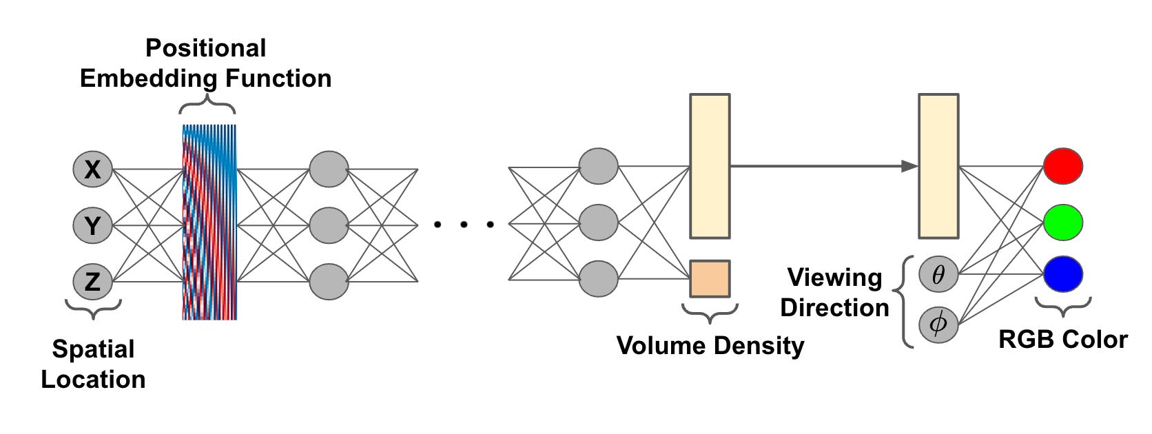
The network takes a 5D coordinate as input—a 3D location $\mathbf{x}=(x,y,z)$ and a 2D viewing direction $\mathbf{d}=(\theta ,\varphi )$—and outputs a 4D value: an RGB color $\mathbf{c}=(r,g,b)$ and a volume density $\sigma$.

This simple but powerful concept is visualized below.

To get a feel for the problem NeRF addresses and its motivation, let's watch a short segment from a presentation by Matthew Tancik, one of the original NeRF authors. He begins by highlighting the limitations of traditional grid-based methods, a topic that should be familiar from our last lesson.

2. The NeRF Architecture

The specific design of the NeRF MLP is intentional and crucial for capturing realistic scenes. As mentioned, density ($\sigma$) should ideally only be a function of location, while color ($\mathbf{c}$) can change depending on the viewing angle (e.g., reflections on a shiny surface).

To achieve this, the NeRF architecture processes the inputs in stages:

1. The 3D position $\mathbf{x}$ is passed through a series of MLP layers.
2. These layers produce the volume density $\sigma$ and an intermediate feature vector.
3. The feature vector is then concatenated with the 2D viewing direction $\mathbf{d}$.
4. This combined vector is passed through additional layers to produce the final RGB color $\mathbf{c}$.

This structure ensures that density is view-independent while color can be view-dependent.

3. The "Secret Sauce": Positional Encoding

If you were to implement the MLP as described so far, you would find the results to be disappointingly blurry. Standard MLPs have a "spectral bias," meaning they are inherently better at learning low-frequency functions and struggle to represent the sharp, high-frequency details found in real-world images.

The authors of NeRF overcame this with a clever trick: positional encoding. Before being fed to the network, the continuous input coordinates ($x,y,z$ and $\theta ,\varphi$) are mapped to a higher-dimensional feature space using a set of sine and cosine functions of varying frequencies.

This isn't the same as positional encoding in Transformers, which encodes discrete positions in a sequence. Here, it helps the MLP to reason about the input coordinates at multiple scales, making it far easier to learn high-frequency variations in color and geometry.

The following segment provides an excellent and intuitive explanation of why this is so effective, using a simple 2D image-fitting task as an example.

4. The Rendering Process: From a Field to Pixels

Now that we have a function $F_{\theta }$ that represents our scene, how do we use it to create an image? The answer is volume rendering.

The intuition is to simulate the physics of light transport. For each pixel in our target image, we trace a camera ray $\mathbf{r}(t)=\mathbf{o}+t\mathbf{d}$ from the camera origin $\mathbf{o}$ in the direction $\mathbf{d}$ through that pixel. The color of the pixel is the accumulated color of all the tiny particles of light that the ray passes through in the scene.

This process is formalized by the volume rendering integral:

Where:

• $\mathbf{C}(\mathbf{r})$ is the final color for the ray $\mathbf{r}$.
• $\sigma (\mathbf{r}(t))$ and $\mathbf{c}(\mathbf{r}(t),\mathbf{d})$ are the density and color at point $t$ along the ray, as predicted by our NeRF MLP.
• $T(t)$ is the transmittance, which represents the probability that the ray travels from the near bound $t_n$ to the point $t$ without hitting anything. It's the accumulated transparency up to that point. It is defined as: $$T(t)=\exp \left(-{\int }_{t_n}^t\sigma (\mathbf{r}(s))ds\right)$$

In practice, we can't compute this continuous integral directly. Instead, we approximate it using a discrete sum, a technique known as numerical quadrature. We sample $N$ points along the ray and sum their contributions. The discrete formula, which closely resembles classical alpha compositing from computer graphics, is:

Where:

• ${\mathbf{c}}_i$ is the color of the $i$-th sample.
• ${\alpha }_i=1-\exp (-{\sigma }_i{\delta }_i)$ is the opacity of the $i$-th sample, where ${\delta }_i$ is the distance to the next sample.
• $T_i={\prod }_{j=1}^{i-1}(1-{\alpha }_j)$ is the discrete transmittance, the probability of reaching the $i$-th sample.

The following reading provides an excellent, mathematically rigorous derivation of these equations, starting from first principles. It also shows how the discrete sum is equivalent to alpha compositing.

The most important takeaway is that this entire rendering process—casting rays, querying the network, and composing the results—is fully differentiable. This means we can use gradient descent to optimize the network's weights $\theta$ by minimizing the difference between the rendered pixel colors and the ground-truth pixel colors from our input images.

5. Efficient Rendering: Sampling Strategies

Naively sampling hundreds of points along every single ray for every pixel in an image would be computationally infeasible. NeRF employs a clever two-pass strategy to make this more efficient.

1. Stratified Sampling (Coarse Pass): Instead of sampling at fixed intervals, the ray is divided into $N_c$ uniform bins, and one sample is drawn randomly from within each bin. This ensures that samples are spread out but also that the continuous volume is more broadly explored during training. These $N_c$ samples are passed through a "coarse" MLP.

2. Importance Sampling (Fine Pass): The outputs from the coarse pass give us a rough idea of where the object's mass is located along the ray (i.e., where the weights ${\alpha }_i{T}_i$ are high). A second set of $N_f$ samples is drawn from the ray, this time biased towards these important regions. All $N_c+N_f$ samples are then passed through a separate "fine" MLP to compute the final, high-quality pixel color.

This hierarchical volume sampling strategy focuses computational power where it matters most, allowing for higher quality renderings with fewer total samples.

The following short clip explains this two-network approach.

Conclusion

In this lesson, we have unpacked the core components of Neural Radiance Fields. We've seen how a surprisingly simple MLP, augmented with positional encoding, can represent a complex 3D scene, and how the principles of volume rendering can transform that implicit representation into a photorealistic image.

Key Takeaways:

• A NeRF represents a scene with an MLP that maps a 5D coordinate (3D position + 2D direction) to a 4D output (RGB color + volume density $\sigma$).
• Positional encoding is a crucial technique that allows the MLP to learn the high-frequency details necessary for photorealism.
• Volume rendering is a differentiable process that synthesizes a pixel's color by integrating the color and density contributions of points sampled along a camera ray.
• The continuous rendering integral is approximated with a discrete sum that is equivalent to alpha compositing.
• Hierarchical sampling makes rendering more efficient by using a coarse-to-fine approach to focus sample points on meaningful areas of the scene.

Next Lesson Preview:

Now that we have a solid conceptual grasp of the NeRF rendering pipeline, we will shift our focus to implementation. The next lessons will be hands-on, where we'll build the key components of this pipeline from scratch. We'll start by implementing ray generation for a pinhole camera model, the very first step in turning a pixel coordinate into a ray ready for marching through our scene.