Modeling Everyday Relationships with Linear Functions

Hello! A graph can show that a cost is rising, but a useful model tells you how much it rises and where it starts. Today you’ll turn an everyday pricing rule into a linear function, then read its two key numbers—the slope and intercept—as quantities with real-world meanings. This is a small but important step toward reading the equations used in machine learning.

Set aside about 35–40 minutes, including the two short video selections.

A starting amount and a repeating amount

Imagine a bike-share plan with a $6 weekly membership fee and a charge of $2 for each ride. Let $n$ be the number of rides in a week, and let $C (n)$ be the total weekly cost in dollars.

The membership fee is paid even if you take no rides. Each ride adds another $2, so the model is

C (n) = 2 n + 6.

For three rides, the ride charges total $6, and the membership adds another $6. Thus $C (3) = 12$ dollars.

This has the general slope-intercept form

y = m x + b .

Here $x$ is the input, $y$ is the output, $m$ is the amount added to the output for each one-unit increase in the input, and $b$ is the output when the input is zero. In the bike-share model, $m = 2$ dollars per ride and $b = 6$ dollars. The letters can change: $C (n) = 2 n + 6$ has the same structure as $y = 2 x + 6$ , but its names remind us what the quantities mean.

Watch how a similar model is built from a book-printing setup fee and a charge per copy:

Master Algebra Linear Model Word Problems! How to Construct a Linear Model and Equation Step-by-Step

In “Master Algebra Linear Model Word Problems!”, TabletClass Math builds a total-cost equation from a fixed setup charge and a price per book. Watch for the decision about which quantity is the input.

Watch the problem setup for the two charges. Then skip ahead to the model construction. Focus on why the number of books multiplies the per-copy charge, while the setup charge is added just once.

The transferable idea is not specific to books or rides: a fixed starting amount plus a constant amount per unit gives a linear model.

What slope and intercept look like on a graph

In $C (n) = 2 n + 6$ , setting $n = 0$ leaves $C (0) = 6$ . The graph therefore meets the vertical cost axis at $(0, 6)$ . That point is the vertical intercept, often called the $y$ -intercept even when the output has another name.

Now increase the number of rides from zero to one. Cost increases from $6 to $8. From one ride to two, it increases from $8 to $10. That steady change is the slope. More generally, between two points on a straight line,

m = \frac{change in output}{change in input} = \frac{y _{2} - y _{1}}{x _{2} - x _{1}} .

The units matter. A slope of $2$ in this example does not mean “$2 total”; it means $2 per additional ride.

The following image shows a useful contrast: a rental with a per-day charge but no starting fee.

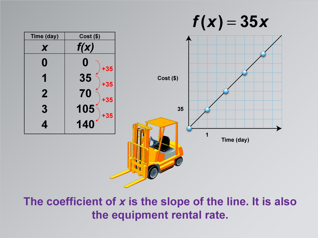
A forklift rental costs \$35 per day: the table increases by \$35 for each additional day, and the graph starts at $(0,0)$. Thus the slope is \$35 per day and the intercept is \$0.

The pictured function is $f (x) = 35 x$ , where $x$ is rental time in days. Its intercept is zero because the pictured model assigns zero cost to zero days. The bike-share line instead starts at $6 because the membership fee applies at zero rides. In both cases, the slope describes the same change each time the input increases by one unit.

Building a model when you are given observations

Sometimes a problem states the fixed fee and per-unit charge directly. Other times, you have to discover them from data. Suppose a bike-share bill shows $8 for one ride and $12 for three rides, and you are told the pricing rule is linear.

The two observations give the points $(1, 8)$ and $(3, 12)$ . Over the additional two rides, cost increases by $4. Dividing the cost change by the ride change gives

m = \frac{12 - 8}{3 - 1} = \frac{4}{2} = 2 dollars per ride .

So far, we know $C (n) = 2 n + b$ , but we do not know the starting fee just by looking at either bill. Substitute the first observation:

8 = 2 (1) + b .

Subtracting $2$ shows that $b = 6$ . Our model is $C (n) = 2 n + 6$ . As a check, three rides should cost $2 (3) + 6 = 12$ dollars, matching the other bill.

This suggests a reliable modeling routine:

Name the input and output, including their units.
Find the constant change per input unit; that is the slope.
Find the output at input zero, either directly or by using a known point; that is the intercept.
Check the model against an observation and say what both numbers mean in context.

The last step prevents a common mistake: reporting “slope $2$ , intercept $6$ ” without saying $2 per ride and $6 with zero rides.

Because rides come in whole numbers, the practical inputs here are $0, 1, 2, \dots$ . A straight line is a convenient picture of the pricing rule, but a value such as $n = 1.5$ does not represent a possible ride count.

An intercept need not be a fee

The intercept always means the modeled output at input zero. Whether that is a fee, a starting balance, or something else depends on what you chose to measure.

Suppose you spend $8 on materials for a lemonade stand and receive $2 for every cup sold. If we count only that stated expense, net money after the materials cost is

P (n) = 2 n - 8,

where $n$ is cups sold and $P (n)$ is dollars. The slope is $2$ dollars per cup. The intercept is $- 8$ dollars: with zero cups sold, you are $8 below where you started. It would be incorrect to call $- 8$ “sales revenue”; revenue and net money after the expense are different outputs.

Watch a visual explanation of this example:

An Intro to Slope-Intercept Form | y=mx+b

In “An Intro to Slope-Intercept Form,” Math with Mr. J uses a lemonade stand to show why a starting expense produces a negative intercept even though each sale adds money.

Watch the lemonade example. Pay particular attention to the starting point at zero cups and the $2 rise per cup. To keep the quantities distinct, read the graphed output as money remaining after the stated $8 expense, rather than sales revenue alone.

A slope can also be negative. If a data allowance begins at $20$ GB and you use a steady $2$ GB per day, a simple model for the amount remaining is

D (t) = 20 - 2 t,

where $t$ is days since the start. Its intercept is $20$ GB, and its slope is $- 2$ GB per day: each additional day leaves $2$ GB less. This model is meaningful only while its assumptions hold—for example, it should not be used to predict a negative amount of data after the allowance runs out.

Linear means the change per input unit stays constant within the model. It does not mean the output must increase, or that the model remains realistic forever.

A small NumPy check

Do the reasoning by hand first; use code to check the values, not to decide what the slope and intercept mean. For the bike-share model, the hand-built table at zero, one, three, and five rides should contain costs of $6, $8, $12, and $16.

import numpy as np

rides = np.array([0, 1, 3, 5])
cost = 2 * rides + 6
print(cost)  # [ 6  8 12 16]

The array calculation applies the same rule to several inputs. It confirms the arithmetic; the pricing story is what tells you that $2$ means dollars per ride and $6$ means the weekly fee.

Takeaways

A linear function packages two ideas: an intercept, the output at zero input, and a slope, the constant output change per input unit. To model a real situation, define what is being measured before assigning meaning to either number, and check whether a constant rate is a reasonable assumption.

Next, you’ll compare the shapes of linear graphs with quadratic and exponential ones. The constant-change pattern you can now recognize will be your reference point.