Limitations of Mean-Variance Optimization

1. The Core Problem: "Garbage In, Garbage Out"

The entire Mean-Variance Optimization framework rests on three key inputs:

1. Expected returns for each asset ($\mu$)
2. Volatilities (standard deviations) for each asset ($\sigma$)
3. The correlation matrix for all assets ($\rho$)

The fundamental problem is that we don't know the true, future values of these parameters. We have to estimate them, usually from historical data. And this is where the trouble begins.

Financial data has several "stylized facts" that make simple statistical estimation based on past data highly problematic. The following video gives an excellent overview of these challenges from a financial engineering perspective.

The key takeaway is that the assumptions we often make to simplify our math (like assuming returns are normally distributed and that the future will resemble the past) are fundamentally flawed. Our estimates of $\mu$ and $\Sigma$ (the covariance matrix) are therefore inherently noisy and potentially biased. This is the "Garbage In" part of the problem.

This creates a significant gap between the theoretical "true" efficient frontier (which is unknowable) and the one we estimate from our flawed data.

The document below provides a powerful visual illustration of this problem.

2. The Optimizer as an "Error Maximizer"

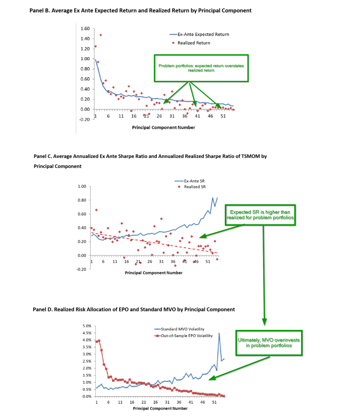
The problem gets worse. The MVO process isn't just a passive user of its inputs; it actively seeks out and exploits the quirks in the data. This means it has a tendency to latch onto assets with the most extreme (and likely erroneous) estimated parameters. An asset that looks unusually good on paper (high estimated return, low correlation) will receive a very large weight in the "optimal" portfolio.

In effect, the optimizer acts as an error maximization machine.

This leads to two well-known practical failures of naive MVO:

• Instability: Small changes to the input estimates can cause wild, dramatic swings in the recommended portfolio weights.
• Unintuitive Portfolios: The model often suggests extreme portfolios, with huge long positions in some assets and huge short positions in others, that no prudent investor would actually implement.

For a more rigorous explanation, consider the work of Best and Grauer (1991), mentioned in the Columbia University paper you just looked at. They showed that the sensitivity of portfolio weights to errors in the mean return vector grows with the condition number of the covariance matrix (the ratio of its largest to smallest eigenvalue, ${\gamma }_{\max }/{\gamma }_{\min }$). As you add more assets to a portfolio, this ratio tends to get very large, making the optimization results extremely sensitive to even tiny estimation errors.

3. Towards a More Robust Framework

Recognizing these flaws doesn't mean we abandon the MVO framework. Instead, practitioners have developed a range of techniques to make it more robust and practical. These methods generally fall into three categories.

The following resource provides an excellent, structured overview of these techniques. We will use it as a guide for this section.

A. Improving the Inputs: Shrinkage and Robust Estimation

Since our sample estimates are unreliable, we can try to create better ones.

Shrinkage Estimation is a key technique. The idea is to take the noisy sample estimate and "shrink" it towards a more stable, sensible target. This introduces a small amount of bias but can dramatically reduce the estimation error (variance), leading to a better overall estimate.

Robust Estimation is an alternative approach that is less sensitive to the "heavy tails" we saw in the first video. Instead of assuming a normal distribution, these methods are designed to be less influenced by extreme outliers.

The following clip shows a compelling visual of how a robust estimator correctly identifies the true data structure while a standard sample estimator is pulled astray by a few outliers.

B. Improving the Model: Using Constraints as Regularization

Another powerful technique is to add constraints to the optimization problem. While constraints like "no short-selling" have obvious practical motivations, they also have a very useful side effect: they regularize the solution and prevent the optimizer from reaching for extreme weights. Imposing a no-short-sale constraint is mathematically similar to shrinking the inputs.

C. Improving the Optimization: Resampling

Finally, rather than trying to perfect the inputs for a single optimization run, we can embrace the uncertainty. Resampled portfolio optimization, pioneered by Richard and Robert Michaud, runs the MVO process hundreds or thousands of times on slightly different versions of the historical data (generated via bootstrapping).

The final portfolio is an average of all these individual "optimal" portfolios. This process tends to average out the estimation errors, leading to a more stable and diversified final allocation that performs better out-of-sample.

Conclusion

In this lesson, we've taken a necessary and critical look at the foundations of the mean-variance framework, completing the first module of our course.

Key Takeaways:

• Naive Mean-Variance Optimization often fails in practice due to two core issues: estimation error (the inputs are noisy) and input sensitivity (the optimizer magnifies those errors).
• Financial return data is not "well-behaved"; its properties like non-stationarity and heavy tails make historical data a poor guide to the future and violate the assumptions of simple statistical models.
• Practitioners use several techniques to make MVO more robust. These include:
  • Improving inputs using shrinkage (e.g., Ledoit-Wolf) and robust estimators.
  • Constraining the model (e.g., no short-selling), which acts as a form of regularization.
  • Improving the optimization process itself through techniques like resampling.

You now have a complete, albeit introductory, understanding of the classic portfolio construction framework, from its theoretical elegance to its practical pitfalls. You are equipped not just to use the model, but to think critically about its results.

In our next module, "The Mechanics of Stock and Bond Returns," we will take a crucial step toward creating better inputs for these models. Instead of relying purely on historical statistical averages for expected returns, we will start building forward-looking estimates by examining the fundamental drivers of asset class returns—namely, earnings growth and valuation changes for stocks, and yield and interest rate changes for bonds.