Building & Understanding the Two-Asset Efficient Frontier

1. The Feasible Set and the "North-West" Rule

Imagine you have two assets, say a stock ETF and a bond ETF. You can allocate your capital between them in countless ways: 100% stocks, 100% bonds, 50/50, 70/30, and so on. Each combination creates a unique portfolio with its own expected return and volatility. If we plot all these possible portfolios on a graph with risk (volatility) on the x-axis and return on the y-axis, we get what is called the feasible set.

So, which portfolio from this set should a rational investor choose? The choice is governed by a simple, intuitive principle.

To understand this principle and the formal definition of the efficient frontier, please read the following sections from the provided PDF on Portfolio Theory.

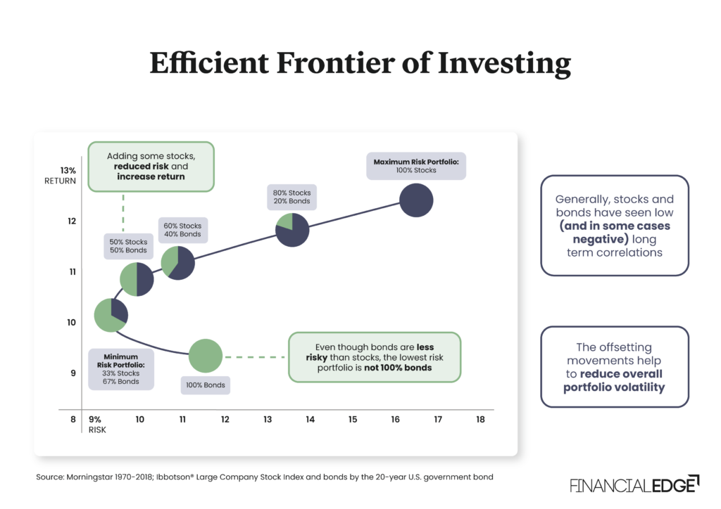
As the text explains, a rational, risk-averse investor will always prefer a portfolio that lies to the "North-West" of another—that is, one with a higher return for the same level of risk, or lower risk for the same level of return. The efficient frontier is the curve representing all portfolios that are not dominated by any other; no other portfolio lies to their North-West.

2. The Mathematics of a Two-Asset Frontier

Let's ground this in the mathematics you prefer. For a two-asset portfolio (Asset A and Asset B), we can define the portfolio's return and variance as a function of a single variable, $w_A$, the weight of Asset A (since $w_B=1-w_A$).

The formulas, which build directly on our last lesson, are:

Portfolio Return:
${\mu }_p=w_A{\mu }_A+(1-w_A){\mu }_B$

Portfolio Variance:
${\sigma }_p^2=w_A^2{\sigma }_A^2+(1-w_A{)}^2{\sigma }_B^2+2w_A(1-w_A){\sigma }_A{\sigma }_B{\rho }_{AB}$

Here, $\mu$ is the expected return, $\sigma$ is the volatility (standard deviation), and ${\rho }_{AB}$ is the correlation coefficient between the returns of Asset A and Asset B.

Notice that the variance formula is a quadratic equation with respect to $w_A$. This is what gives the efficient frontier its characteristic curved shape (a hyperbola). The degree of curvature is heavily influenced by the correlation, ${\rho }_{AB}$. The lower the correlation, the more the curve bends to the left, offering greater diversification benefits.

3. Pinpointing the Minimum Variance Portfolio

A key point on this curve is its vertex—the leftmost point, which represents the portfolio with the lowest possible risk. This is called the Minimum Variance Portfolio (MVP).

Since the portfolio variance, ${\sigma }_p^2$, is a quadratic function of the weight $w_A$, we can find the weight that minimizes it using calculus: by taking the derivative of the variance equation with respect to $w_A$ and setting it to zero.

The following video provides a clear, step-by-step derivation of the weights for the Minimum Variance Portfolio.

4. Constructing the Frontier in Practice

Now that you understand the theory and the underlying math, let's walk through the process of constructing an efficient frontier from scratch using historical data in Excel. This aligns with your preference for hands-on, quantitative tasks.

The following video will guide you through:

1. Calculating the necessary inputs (average returns, volatilities, covariance) for two assets.
2. Creating a table of different portfolio weights.
3. Calculating the portfolio return and volatility for each weight combination using the formulas we discussed.
4. Plotting these points to visually generate the efficient frontier.

As you watch, notice how the plotted points form the characteristic curve. The top half of this curve is the efficient frontier. Any portfolio on the bottom half is "sub-optimal" because there is a portfolio on the top half that offers a higher return for the exact same amount of risk.

5. Interpreting the Frontier: The Power of Diversification

You have now seen the definition, the math, and the practical construction of an efficient frontier. The final step is to solidify its interpretation.

The curved shape of the frontier is the visual proof of diversification. If two assets were perfectly correlated ($\rho =1$), the graph would be a straight line between them. The fact that it bends to the left shows that by combining assets that don't move in perfect lockstep, you can create a portfolio with lower risk than a simple weighted average of the individual assets' risks.

The Efficient Frontier of Investing image above perfectly illustrates this. Notice that the minimum risk portfolio is not 100% in bonds (the least risky asset) but a mix of stocks and bonds. By adding a small amount of a riskier, uncorrelated asset (stocks), the overall portfolio volatility decreases. This is a non-intuitive but powerful result of modern portfolio theory.

Portfolios on the efficient frontier are considered optimal in a mean-variance sense. The choice of which portfolio to pick on the frontier depends on an individual investor's risk tolerance. An investor who is highly risk-averse might choose a portfolio near the Minimum Variance Portfolio. An investor seeking higher returns (and willing to accept more risk) would move further up and to the right along the curve.

Conclusion

In this lesson, we moved from analyzing a single portfolio to mapping the entire set of optimal possibilities.

Here are the key takeaways:

• The efficient frontier represents the set of portfolios that offer the highest possible expected return for a given level of risk.
• It is constructed by plotting the risk and return of all possible weight combinations of the assets in a portfolio. For two assets, this creates a hyperbolic curve.
• The curved shape of the frontier visually demonstrates the benefits of diversification, which are greatest when assets have low correlation.
• Key points on the frontier include the Minimum Variance Portfolio, which can be found precisely using calculus.
• A rational, risk-averse investor should only consider portfolios that lie on the efficient frontier.

We have now identified the set of "best" possible portfolios. But the frontier contains infinitely many points. How do you choose the single best one?

In our next lesson, we will answer that question by introducing a risk-free asset. Combining a risk-free asset with the portfolios on the efficient frontier will allow us to identify a single "optimal risky portfolio" and evaluate any portfolio's performance using a powerful risk-adjusted return metric: the Sharpe ratio.