In our previous lesson, we constructed the full Variational Autoencoder loss function, understanding it as a delicate balance between two competing objectives: accurate data reconstruction and a well-regularized latent space. This tension, governed by the reconstruction and KL divergence terms, is the very source of a VAE's generative capabilities. However, it's also the origin of its characteristic failure modes.
Today, we will investigate these failure modes. Our focus will be on two of the most well-known issues: the tendency for VAEs to produce blurry images and the more subtle but critical problem of posterior collapse. By dissecting why these problems occur, we not only gain a deeper appreciation for the VAE framework but also build the motivation for the architectural innovations we will see in diffusion models later in the course.
The Blurry Output Problem
One of the first things you might notice when comparing samples from a VAE to those from other generative models, like Generative Adversarial Networks (GANs), is a distinct lack of sharpness. VAE-generated images often appear blurry or fuzzy.

This blurriness is not an accident; it's a direct consequence of the VAE's objective function. Let's break down the reasons:
-
The "Averaging" Effect of MSE Loss: In the last lesson, we saw that when modeling real-valued data like image pixels, the reconstruction loss often simplifies to the Mean Squared Error (MSE) between the input and the output. MSE is a pixel-wise distance metric. Consider a single latent point that could plausibly decode to several slightly different, but all sharp, versions of an image (e.g., a face with eyes open vs. eyes slightly squinted). To minimize the average MSE over all these possibilities, the decoder's optimal strategy is to output the average of all those sharp images. The average of many sharp but slightly different images is a blurry one.
-
Inadequacy of Pixel-wise Loss: The MSE loss function is not a good proxy for human perceptual similarity. It heavily penalizes small shifts or rotations in an image, even if the image content is identical. This pressure encourages the decoder to find "safe," low-variance solutions, which often means predicting the mean color (greyish tones) in areas of high uncertainty, contributing further to the blur.
-
The Role of the Encoder and KL Regularization: The encoder is trained to map similar inputs to nearby points in the latent space. The KL divergence term then regularizes this space, encouraging it to be smooth and continuous. This makes it difficult for the model to "memorize" fine details. To produce a perfectly sharp output, the encoder would need to produce a highly specific latent code, and the decoder would need to map that code to a single, sharp image. The KL pressure against creating such specific, potentially isolated representations in the latent space can indirectly contribute to the decoder's averaging behavior.
In an interesting preview of where we are heading, this issue of blurry samples is one reason why diffusion models, which can be viewed as VAEs with a fixed non-learnable encoder, can produce sharper samples. Learning the encoder and decoder jointly can sometimes lead to better loss values on paper (a higher ELBO) but result in poorer sample quality.
Stanford CS236: Deep Generative Models I 2023 I Lecture 16 - Score Based Diffusion Models
This segment from a Stanford lecture on score-based models touches upon this exact point. It explains that while learning the encoder might seem optimal, it doesn't always work well in practice and can lead to blurry samples, a classic VAE characteristic.
Please watch the section from this timestamp. The lecturer discusses how jointly learning the encoder and decoder can yield better ELBO values but worse sample quality, specifically mentioning "blurry samples" as a typical VAE outcome.
Posterior Collapse
A more fundamental and damaging failure mode in VAEs is posterior collapse. This occurs when the latent variables become uninformative, meaning the decoder learns to ignore them entirely.
Formally, posterior collapse happens when the approximate posterior collapses onto the prior for every input .
When this happens, the KL divergence term goes to zero. This is an "easy win" for the optimizer, but it comes at a great cost: the latent code no longer contains any information about the input . The encoder effectively stops encoding. Consequently, the decoder learns to generate the single best reconstruction it can without any information from z—which is typically the average of all images in the training set. The model loses all ability to reconstruct specific inputs or generate diverse new samples.
The Cause: An Unbalanced Competition
Posterior collapse is the result of the competition between the reconstruction term and the KL regularization term.
- The KL term wants to make as simple as possible, pushing it towards the prior .
- The reconstruction term needs an informative from the encoder to accurately reconstruct .
The collapse happens when the balance tips too far in favor of the KL term. This is especially likely if the decoder is very powerful (e.g., a deep autoregressive network). A powerful decoder might be able to model the data distribution reasonably well on its own, without conditioning on . In this case, the path of least resistance for the overall optimization is to let the KL term go to zero (by ignoring ) and have the decoder do all the heavy lifting.
For a mathematically rigorous understanding of this phenomenon, we can turn to a simplified linear VAE model, where the dynamics of collapse can be analyzed precisely.
[PDF] Posterior Collapse of a Linear Latent Variable Model
This paper provides a brilliant analysis of posterior collapse. By studying a linear VAE, the authors derive the exact conditions under which collapse occurs, revealing that it's a competition between the signal strength in the data and the regularization imposed by the prior.
Start by reading the Introduction to understand the problem statement. Then, review the model setup in the brief section right after the introduction, focusing on Equation (1), which presents the ELBO. Next, jump to Section 4.2, "Linear VAE without Learnable Σ". This is the core of the analysis. Pay close attention to Theorem 1 and the discussion that follows. It identifies the critical condition for collapse: \zeta_i - \sqrt{\beta \eta_{dec}} \le 0, where \zeta_i is related to the data's principal components (signal strength), \eta_{dec} is the decoder variance, and \beta is the weight on the KL term. This shows that if the regularization (\beta) is too strong relative to the signal, the latent dimension collapses. Then, read the analysis in Section 4.3, "Linear VAE with Learnable Σ". The key takeaway here is that even with a learnable latent variance, the fundamental condition for collapse remains the same. Finally, look at Figure 3 in Section 5, "Numerical Examples". This figure provides a powerful visual demonstration of the theory. As \beta increases, more latent dimensions collapse, and the generated MNIST digits lose diversity, eventually collapsing to a single blurry average.
The analysis in the paper makes it clear: posterior collapse is not just a quirk of complex models but a fundamental property of the VAE objective. The hyperparameter (often implicitly 1 in the standard VAE loss) plays a crucial role in mediating this trade-off. If it's too high, it encourages the model to discard information from the data in favor of matching the prior.
Mitigating VAE Failure Modes
Given that these issues are inherent to the VAE objective, several techniques have been developed to manage them.
KL Annealing
The most common method to prevent posterior collapse is KL annealing. The idea is to start training with the weight of the KL term, , set to 0 and gradually increase it to 1 over a number of training epochs.
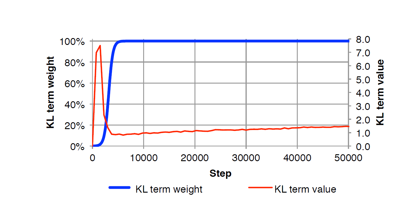
This "warm-up" phase forces the model to focus exclusively on the reconstruction loss first. The encoder must learn to pass useful information to the decoder to reconstruct the inputs. Once this meaningful latent representation is established, the KL regularization is slowly introduced to structure the latent space without causing it to collapse.
The paper "Understanding Posterior Collapse in Generative Latent Variable Models" discusses the role of KL annealing and other factors.
Understanding Posterior Collapse in Generative Latent ...
This paper provides further context on posterior collapse, reviewing common mitigation techniques and arguing that spurious local maxima in the objective landscape are a key cause.
Please read the section on KL-annealing in Section 5.2. The authors note that while it provides temporary relief, the posterior may still collapse once regular training resumes if other factors (like the decoder's variance, \sigma^2) are not well-tuned. Also, briefly review the first half of Section 5.2, "Training with fixed σ^2", which demonstrates empirically how a poorly chosen decoder variance can lead to collapse, while a smaller variance allows the model to learn better representations.
Architectural Solutions: The VQ-VAE
Another way to address these failures is to change the architecture itself. The Vector-Quantized VAE (VQ-VAE) is a fascinating variant that completely avoids the posterior collapse problem by using a discrete latent space and a different loss structure.
Instead of mapping an input to a continuous distribution, the VQ-VAE encoder maps it to the closest vector in a learned, finite "codebook." Because the KL divergence term (which drives the collapse) is either constant or non-existent in this formulation, the model is not pushed to ignore the latent code. This architecture also tends to produce sharper images because the decoder is trained on a set of discrete, well-defined latent codes rather than a continuous, potentially "averaged" space.
Vector-Quantized Variational Autoencoders (VQ-VAEs) | Deep Learning
This video by DeepBean provides an excellent explanation of the VQ-VAE. This particular section details its unique loss function, which is key to understanding how it sidesteps the issues we've discussed.
Watch the segment on the loss function. It explains the three components: reconstruction loss, codebook loss, and commitment loss. Notice how this structure replaces the KL divergence term, instead using the commitment loss to ensure the encoder doesn't stray too far from the learned codebook vectors, preventing a form of collapse while encouraging the codebook to be well-utilized.
Conclusion
In this lesson, we've explored the inherent trade-offs in the VAE objective that lead to its most common failure modes.
Here are the key takeaways:
- Blurry outputs are primarily a consequence of using pixel-wise loss functions like MSE, which incentivize the decoder to produce "average" reconstructions rather than sharp, perceptually realistic ones.
- Posterior collapse occurs when the KL regularization term overwhelms the reconstruction objective, causing the model to learn uninformative latent variables and ignore the input data. This is especially prevalent when using powerful decoders.
- The balance between reconstruction and regularization, often controlled by the KL weight , is critical. A that is too large relative to the signal strength in the data can trigger collapse.
- Techniques like KL annealing are common heuristics to mitigate posterior collapse by giving the encoder a head start on learning a useful representation.
- Architectural changes, like the discrete latent space in VQ-VAEs, can fundamentally solve the posterior collapse problem by reformulating the training objective.
Understanding these weaknesses is crucial. It not only helps in debugging and training VAEs effectively but also provides the motivation for the development of more advanced generative models. In our next lesson, we will put this theory into practice by implementing and training a VAE in PyTorch, where we will have the chance to observe some of these behaviors firsthand.