Advanced SQL: Joins, Grouping, and Aggregation

1. Reconstructing Data with JOIN Clauses

Normalization required you to place book information in a books table and chapter information in a chapters table, linked by a foreign key like book_id. A JOIN clause is the mechanism that traverses this link, creating a single, virtual table from two or more physical tables.

There are several types of joins, but the most essential are:

• INNER JOIN: This is the most common type of join. It returns only the rows where the join condition is met in both tables. If you join books and chapters on books.id = chapters.book_id, you will only get results for books that have at least one chapter.
• LEFT JOIN (or LEFT OUTER JOIN): This returns all rows from the left-hand table and the matched rows from the right-hand table. If there's no match for a row from the left table, the columns from the right table will be filled with NULL. This is invaluable for asking questions like, "Show me all books, and if they have chapters, list them." A book with no chapters would still appear, but its chapter-related columns would be NULL.
• RIGHT JOIN and FULL OUTER JOIN: These are logical extensions. RIGHT JOIN is the inverse of LEFT JOIN (all rows from the right table), and FULL OUTER JOIN returns all rows from both tables, inserting NULLs where matches don't exist on either side.

To understand the precise syntax and structure, the PostgreSQL official documentation is the canonical source.

2. Under the Hood: Join Algorithms

Simply writing a JOIN is declarative—you state what you want. The database's query optimizer then decides how to execute it. This is a critical distinction for an engineer. The optimizer chooses from several algorithms, each with different performance characteristics. Understanding these provides the foundation for query tuning, a topic we will cover in depth later.

The three canonical join algorithms are:

1. Nested Loop Join: The most basic approach. The database iterates through every row of the first (outer) table and, for each of those rows, scans the entire second (inner) table looking for matches. The naive version is $O(M\times N)$, which is terribly slow, but variants that use memory blocking (Block Nested Loop Join) or indexes (Index Nested Loop Join) are far more efficient and are often used for small joins.
2. Sort-Merge Join: This algorithm works in two phases. First, it sorts both tables on the join key. Second, it merges the two sorted lists, advancing pointers through each list in a synchronized way. This is highly efficient if the tables are already sorted on the join key or if the final output needs to be sorted anyway.
3. Hash Join: This is often the fastest algorithm for large, unsorted equi-joins. It also has two phases: a "build" phase, where it scans the smaller table and builds an in-memory hash table on the join key, and a "probe" phase, where it scans the larger table, hashing its join keys to find matches in the hash table.

To get a high-level intuition, the following lecture from CMU's Intro to Database Systems course is an excellent starting point.

For a deeper, more rigorous examination of the I/O costs and implementation details—which is essential for your goal of mastery—the following lecture slides provide the necessary engineering detail.

3. Summarizing Data with GROUP BY

Once you have joined tables to get a comprehensive set of rows, the next step is often to compute summaries. For instance, you don't just want a list of all chapters for all books; you want to know the count of chapters per book.

This is the job of the GROUP BY clause. It takes a large set of rows and partitions them into smaller groups based on the values in one or more columns.

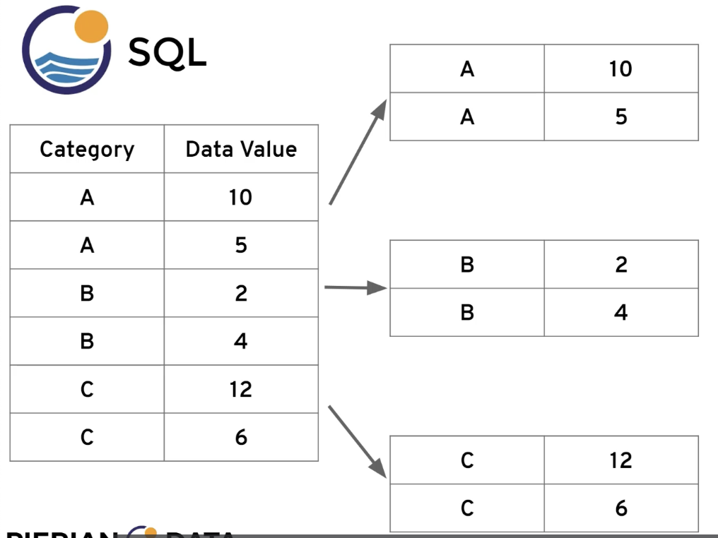
Once the data is grouped, you can apply aggregate functions to each group. Common functions include:

• COUNT(): Counts the number of rows in the group.
• SUM(): Sums the values in a column for the group.
• AVG(): Calculates the average value.
• MIN() / MAX(): Finds the minimum or maximum value.

To filter these newly formed groups, you cannot use WHERE. The WHERE clause filters rows before they are grouped. To filter after grouping, you must use the HAVING clause. For example, to find books with more than 20 chapters, you would first group by book and count the chapters, then use HAVING COUNT(*) > 20.

This distinction highlights the logical order of query processing in SQL, a crucial first principle. Although you write SELECT first, the database logically processes clauses in this order:

1. FROM and JOIN: Assembles the initial set of rows.
2. WHERE: Filters individual rows.
3. GROUP BY: Partitions the remaining rows into groups.
4. HAVING: Filters entire groups.
5. SELECT: Computes the final output columns.
6. ORDER BY: Sorts the final result set.
7. LIMIT: Restricts the number of rows returned.

Understanding this order explains why you can't use a column alias defined in the SELECT list within a WHERE clause—the WHERE clause is evaluated before the SELECT list!

The official documentation provides the complete syntax.

Just as with joins, databases have different algorithms for aggregation, primarily falling into two camps: sorting-based (sort the data by the group key, then iterate) and hashing-based (build a hash table to accumulate results for each group). The CMU video on aggregations explains this internal logic.

4. Your Task: Querying the Narrative Database

Now, apply these concepts to the schema you designed in the previous lesson. Create a new SQL file in your project repository (e.g., queries.sql) and write the following queries. Assume you have populated your tables with some sample data representing a few books, each with multiple chapters and chunks.

1. Simple Join: Write a query that joins your books, chapters, and chunks tables (or navigates your adjacency list documents table) to retrieve the content of all chunks belonging to the book titled 'Dune'.
2. Join with Aggregation: Write a query that calculates the number of chunks for each chapter in the book 'Dune'. The output should include the book title, chapter number, chapter title, and the count of chunks.
3. Complex Aggregation with Filtering: Write a query to find all authors who have written more than one book in your database. The output should be the author's name and the count of their books. This will require joining, grouping by author, and using a HAVING clause to filter the groups.

Commit this file to your repository. In your engineering journal, for each query, briefly explain the purpose of each clause (JOIN, GROUP BY, HAVING) and which join algorithm (Hash, Sort-Merge, Nested Loop) you hypothesize PostgreSQL might choose and why.

Conclusion

In this lesson, you've acquired two of the most powerful tools in the SQL language. You learned to use JOINs to weave together normalized data, reconstructing a complete picture from separate tables. You then learned to use GROUP BY and aggregate functions to distill that data into concise, meaningful summaries. Crucially, you also peered beneath the surface to understand the internal algorithms that databases employ, appreciating that a single line of SQL can trigger complex operations with significant performance trade-offs.

Key Takeaways:

• JOIN clauses (INNER, LEFT) are used to combine rows from multiple tables based on related columns.
• Databases execute joins using algorithms like Nested Loop, Sort-Merge, and Hash Join, chosen by the query optimizer based on table sizes, indexes, and data distribution.
• GROUP BY partitions rows into groups, on which aggregate functions (COUNT, SUM, AVG) can operate.
• WHERE filters rows before aggregation, while HAVING filters groups after aggregation. This is dictated by SQL's logical processing order.

In our next lesson, we will bridge the gap between your database and your application code. You'll learn how to connect to PostgreSQL from a Python application using the psycopg library and execute parameterized queries, a vital skill for building the API for your Narrative Intelligence Engine and a crucial defense against SQL injection attacks.