Determining Sample Size for Estimating Population Mean

From Finding the Best to Estimating the Average

The core of our new hypothesis is a shift from selection to estimation. Instead of trying to pinpoint the single best design, we want to estimate the true average quality score ($\mu$) of all 20 finalist designs. Our tool is the sample mean ($\bar{x}$), calculated from a subset of reviewed designs.

However, any estimate based on a sample comes with uncertainty. The key to a defensible process is to quantify and control that uncertainty. We do this by specifying two things upfront:

1. Confidence Level: How certain do we want to be that our estimation process captures the true mean? (e.g., 95% confidence).
2. Margin of Error ($E$): How much error are we willing to tolerate in our estimate? (e.g., we want our estimated average score to be within $\pm 5$ points of the true average).

A confidence interval gives us a range that likely contains the true population mean. Its general form is:

$\text{Estimate}\pm \text{Margin of Error}$

For a population mean, this looks like:

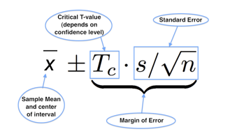
Our goal is to choose a sample size $n$ that makes the margin of error, $E$, as small as we require. This is a classic problem in the Design of Experiments, your area of expertise. The following article provides an excellent introduction to this precision-based approach to sample size.

The Formula for Sample Size

As the article you just read explains, the formula for the margin of error contains the sample size, $n$. We can therefore rearrange it to solve for $n$. The margin of error for estimating a mean is:

$E=z_{\alpha /2}\frac{\sigma }{\sqrt{n}}$

Here:

• $E$ is the desired margin of error.
• $z_{\alpha /2}$ is the critical value from the standard normal distribution for our chosen confidence level.
• $\sigma$ is the population standard deviation of the measurements (in our case, the design scores).
• $n$ is the sample size we need to find.

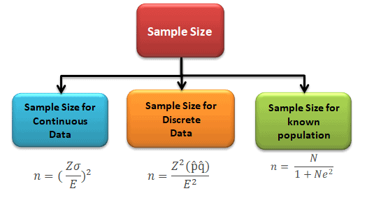
Solving for $n$, we get the fundamental formula for sample size calculation for a mean:

$n={\left(\frac{z_{\alpha /2}\sigma }{E}\right)}^2$

This is the formula for continuous data shown in the diagram below.

Case File: A Defensible Judging Process

Let's build a defensible protocol for the Aphrodite's Veil legal team. They want to be 95% confident that their estimate of the average quality of the 20 finalist designs is within $\pm 5$ points of the true average.

We have our requirements:

• Confidence Level: 95%, which corresponds to a $z_{\alpha /2}$ value of 1.96.
• Margin of Error ($E$): 5 points.

The one missing piece is $\sigma$, the standard deviation of the quality scores. This is a common hurdle—to know the required sample size, you need to know something about the population's variability, which you haven't fully sampled yet!

Fortunately, we have several ways to estimate $\sigma$. A very practical method, especially when prior data is sparse, is the range rule of thumb. The following resource demonstrates this in a worked example.

Now, let's apply this to our case.

1. Estimate $\sigma$: The scores are on a 100-point scale. While the full range is 0-100, the 20 finalists are likely to be clustered at the high end. Let's make a reasonable assumption that the scores for this elite group will fall between 70 and 100.

   • Range = 100 - 70 = 30 points.
   • Using the range rule of thumb from the example: $\sigma \approx \frac{\text{Range}}{4}=\frac{30}{4}=7.5$.

2. Calculate Initial Sample Size ($n_0$): Now we plug our values into the formula.
   $n_0={\left(\frac{z_{\alpha /2}\sigma }{E}\right)}^2={\left(\frac{1.96\times 7.5}{5}\right)}^2=(2.94{)}^2\approx 8.64$
   Since we cannot review a fraction of a design, we must always round up. This gives us an initial sample size of $n_0=9$.

A Final Twist: The Finite Population Correction

The formula we used assumes the population is very large. However, our population of finalist designs is very small ($N=20$). When the sample size is more than 5% of the total population (here, $9/20=45\%$, which is much larger), sampling without replacement starts to reduce the variability. We gain more information from each sample than we would from an infinite population.

We must therefore apply a Finite Population Correction (FPC) to adjust our result. The adjusted sample size $n$ is calculated from our initial estimate $n_0$ and the population size $N$:

$n=\frac{n_0}{1+\frac{n_0}{N}}$

Let's apply this correction to our case:

• $n_0=9$
• $N=20$

$n=\frac{9}{1+\frac{9}{20}}=\frac{9}{1+0.45}=\frac{9}{1.45}\approx 6.2$

Again, we round up to the next whole number. The final required sample size is 7.

This means that by randomly selecting and reviewing just 7 of the 20 designs, the judges could be 95% confident that the average score they calculated is within 5 points of the true average for all 20 finalists. This provides a statistically robust and efficient protocol that is far more defensible than a high-risk gamble.

Conclusion

Today, we've developed a powerful alternative hypothesis. The contest might not have been a high-stakes search for the single best design, but a methodical process of estimation. As an efficiency expert, you can appreciate the elegance of achieving a desired level of precision with the minimum necessary work.

Your key takeaways are:

• Precision-Based Sample Size: We can determine the sample size needed to estimate a population mean by specifying our desired confidence and margin of error.
• The Core Formula: The calculation hinges on the formula $n=(\frac{z\sigma }{E}{)}^2$, which requires an estimate for the population standard deviation, $\sigma$.
• Practical Estimation: The range rule of thumb ($\sigma \approx \text{Range}/4$) is a useful tool for estimating $\sigma$ when prior data is unavailable.
• Finite Population Correction: For small populations, the FPC must be applied to avoid overestimating the required sample size.

We now have two competing, statistically valid strategies that could explain the events of the contest: the 1/e rule to find the best, and a sampling plan to estimate the average. Both result in a decision based on a subset of the data. But which approach is "better"?

Preview of the Next Lesson

To answer that question, we need to move beyond just applying statistical tools and start evaluating the tools themselves. How do we formally compare two different methods, or "estimators"? What makes one estimator superior to another?

In our next session, we will investigate the fundamental properties used to judge statistical estimators: bias, variance, and Mean Squared Error (MSE). This will give us a rigorous framework to compare the "find the best" strategy against the "estimate the average" strategy and get to the heart of what makes for a truly good decision.