Pole-Zero Cancellations and System Modes

From State-Space to Transfer Function: Poles and Zeros

First, let's refresh the relationship between a state-space model and its transfer function. The transfer function $G(s)$ is given by:

As you know from your signal processing work, the poles of $G(s)$ dictate the system's dynamic modes (stability, oscillation frequency, etc.), while the zeros affect the response's shape and magnitude.

A common rule of thumb is that the poles of the transfer function are simply the eigenvalues of the state matrix $A$. But is this always true? The following video provides an excellent and nuanced answer.

The key takeaway from the video is this:

• The eigenvalues of A represent the poles of the system's internal dynamics.
• The poles of the transfer function $G(s)$ represent the poles of the system's input-output behavior.

These two sets are identical if and only if the system is both controllable and observable. If a mode is uncontrollable or unobservable, it will be absent from the transfer function due to a pole-zero cancellation.

The Danger of Hidden Modes

When a pole is cancelled by a zero, that mode becomes "hidden" from the input-output map. This might seem like a convenient simplification, but it can be extremely dangerous if the cancelled pole is unstable.

The following resource illustrates this with a stark example.

As the example shows, the system has an unstable eigenvalue at $\lambda =+2$. This means that for certain initial conditions, the state vector $\mathbf{x}(t)$ will grow without bound. However, because this unstable mode is cancelled in the transfer function, it is invisible at the output $y(t)$. You could be looking at a perfectly well-behaved output signal while the system is internally tearing itself apart.

This is precisely why state-space analysis is so powerful; it reveals the complete internal picture, including these potentially hidden, unstable modes. The process of removing these cancellations to get the simplest input-output representation is called finding a minimal realization. In MATLAB, the minreal function is designed for this purpose, as shown in the video Using ‘minreal’ in Matlab to Perform Transfer Function Pole/Zero Cancellation (resource LINK).

Linking Cancellation to Controllability & Observability

So, how can we tell if a cancellation corresponds to a loss of controllability or observability? The structure of the system provides the answer. Consider a system made of two blocks in series, $G_1(s)$ followed by $G_2(s)$.

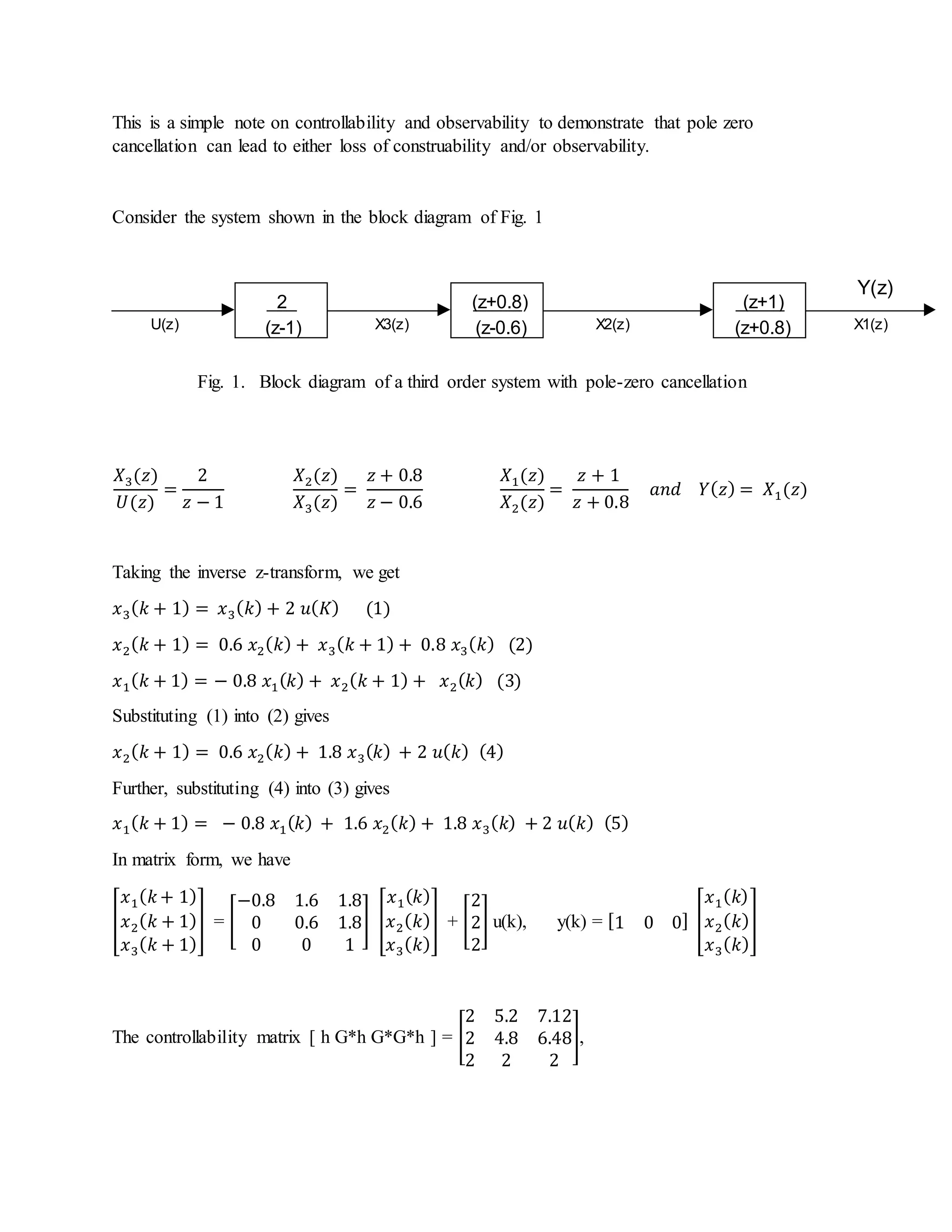
The logic, which applies equally to continuous-time systems, can be understood intuitively:

1. Uncontrollable Mode: A mode becomes uncontrollable if the input signal's path to that mode is blocked. This happens when a zero upstream of a pole cancels it. In the diagram above, the input u(k) is filtered by the first block. If a subsequent block has a zero that cancels a pole from the first block, that pole's dynamic mode was never fully "excited" by the input in a way that can be seen at the final output. The input's influence is nullified.

2. Unobservable Mode: A mode becomes unobservable if its contribution to the output is blocked. This happens when a pole is cancelled by a zero downstream. The state associated with the pole evolves internally, but its effect is filtered out by the subsequent zero before it can ever influence the final output $y(k)$.

This useful rule of thumb is summarized nicely in the document "Controllability and Observability" (resource LINK) under the heading 'Pole Zero Cancellation'.

Pinpointing the Problem: The PBH Test

The rank tests for the controllability and observability matrices tell us if a system has hidden modes, but they don't tell us which specific modes (eigenvalues) are the culprits. For that, we can use a more precise tool.

The Popov-Belevitch-Hautus (PBH) test allows you to check controllability and observability for each eigenvalue ${\lambda }_i$ individually.

• Controllability PBH Test: A mode ${\lambda }_i$ is controllable if and only if the matrix $[A-{\lambda }_{i}IB]$ has full rank ($n$).
• Observability PBH Test: A mode ${\lambda }_i$ is observable if and only if the matrix $\left[\begin{array}{c}A-{\lambda }_{i}I\\ C\end{array}\right]$ has full rank ($n$).

If the rank drops below $n$ for a specific eigenvalue, that is your hidden mode. This is an incredibly useful diagnostic tool, connecting directly to the linear algebra concepts you're familiar with. You can see examples of this test applied to an RC filter and the cart-pendulum system in the resource Controllability and Observability (ID LINK) under the 'PBH Test' section.

Conclusion

Today, we've connected the dots between state-space properties and transfer function analysis. This synthesis is crucial for a deep understanding of control systems.

Key Takeaways:

• Pole-zero cancellation in a transfer function is the input-output signature of an uncontrollable or unobservable mode.
• The system's minimal realization (the transfer function after cancellations) only describes the controllable and observable part of the system.
• An unstable but hidden (unobservable) mode is a significant risk, as the system can be internally unstable while the output appears perfectly fine. State-space analysis is essential for detecting such conditions.
• The structure of the cancellation tells you the nature of the issue: a zero canceling an upstream pole indicates an uncontrollable mode, while a zero canceling a downstream pole indicates an unobservable mode.
• The PBH test provides a precise method to identify which specific eigenvalue corresponds to the uncontrollable or unobservable mode.

Preview of the Next Lesson:

We have now completed our tour of the fundamental properties of dynamic systems. You understand how to model systems, and how to analyze them for stability, controllability, and observability. You are now fully equipped to move into the core topic of this course: multivariable systems. In our next lesson, we will begin Module 3 by learning how to formulate state-space equations for systems with multiple inputs and multiple outputs (MIMO), setting the stage for modeling your rotary inverted pendulum.