State-Space Models from Differential Equations

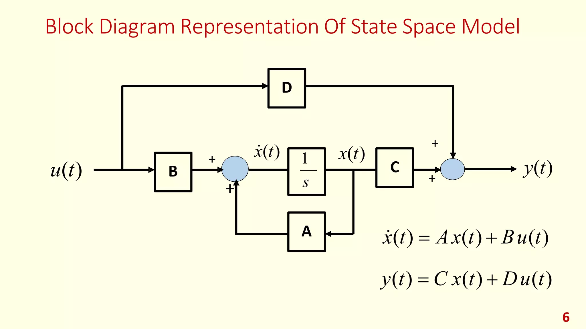
From Nth-Order DE to a System of First-Order Equations

The core idea of a state-space model is to represent a system using only first-order differential equations. So, if we start with a single $n$-th order differential equation, our first task is to break it down into $n$ first-order equations.

The most straightforward way to do this involves defining a chain of state variables, where each new variable is the derivative of the last.

For an $n$-th order differential equation involving a variable $y$, we can define the state variables as:

• $x_1=y$ (the variable itself)
• $x_2=\dot{y}$ (its first derivative)
• $x_3=\ddot{y}$ (its second derivative)
• ...
• $x_n=y^{(n-1)}$ (its $(n-1)$-th derivative)

This clever choice gives us $n-1$ state equations almost for free:

• ${\dot{x}}_1=\dot{y}=x_2$
• ${\dot{x}}_2=\ddot{y}=x_3$
• ...
• ${\dot{x}}_{n-1}=y^{(n-1)}=x_n$

The final equation, for ${\dot{x}}_n=y^{(n)}$, comes from rearranging the original differential equation to solve for its highest derivative.

The following video provides an excellent demonstration of this exact process.

The Resulting Structure: Controllable Canonical Form

When you use this specific method of choosing state variables ($x_1=y,x_2=\dot{y}$, etc.) for a differential equation with no derivatives of the input, the resulting $A$ and $B$ matrices have a very specific and useful structure.

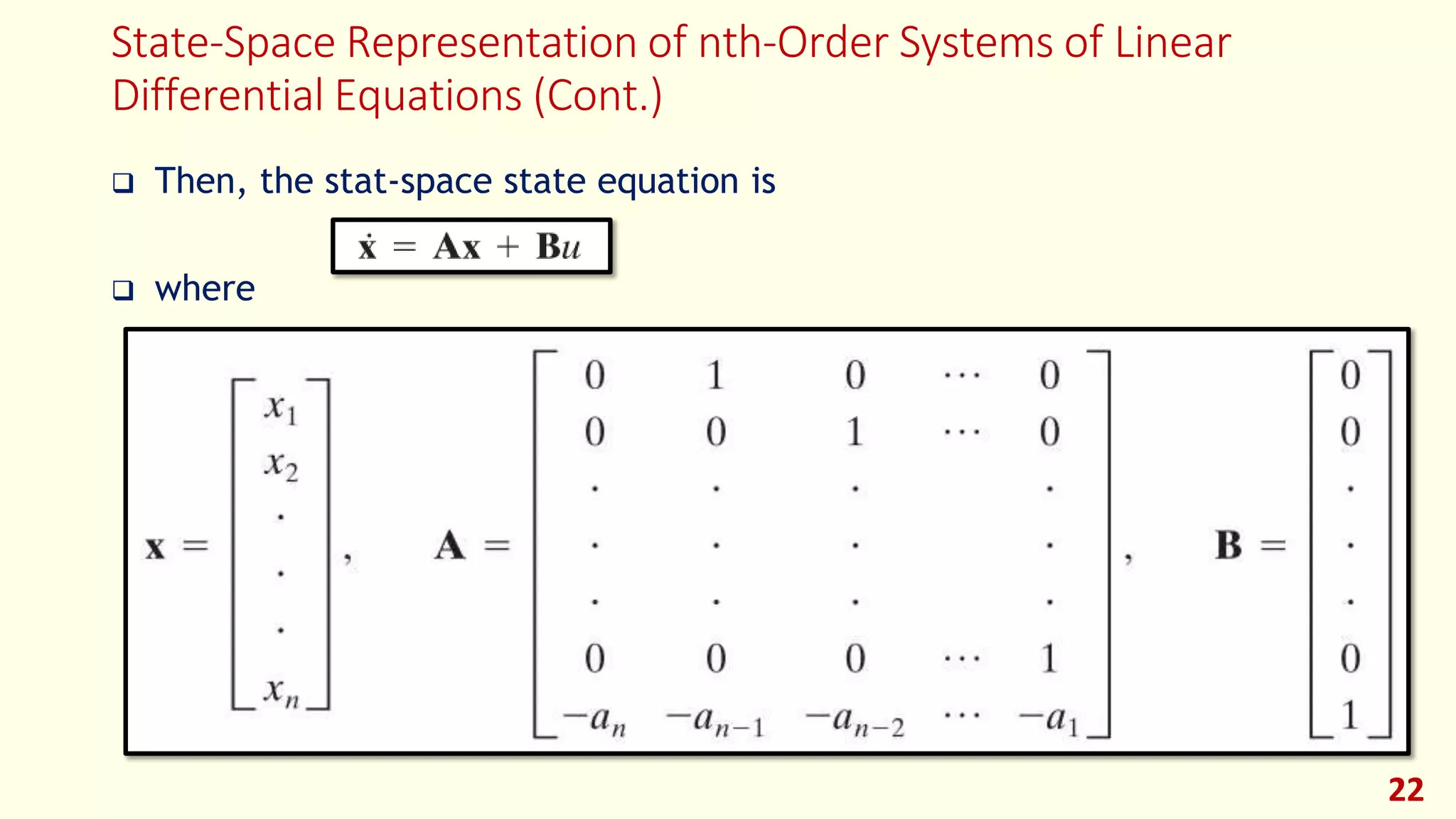
This structure is called Controllable Canonical Form. Recognizing this pattern can be a significant shortcut. Once you've rearranged your differential equation in the standard form (highest derivative on the left), you can often write down the $A$ and $B$ matrices directly by inspection.

From Physical Laws to State-Space Models

More often, instead of starting with a single high-order differential equation, you will start with a physical system. As we saw in the last lesson, you can use physical principles to choose your state variables (inductor currents, capacitor voltages, etc.). You then apply physical laws (Kirchhoff's, Newton's) to write a set of coupled equations and rearrange them into state-space form.

Since your background is in Electrical Engineering, let's focus on an RLC circuit. This approach should feel very natural.

The General Process:

1. Choose State Variables: As per our previous lesson, pick inductor currents and capacitor voltages.
2. Write Dynamic Equations: Apply Kirchhoff's Voltage Law (KVL) for loops containing inductors and Kirchhoff's Current Law (KCL) for nodes connected to capacitors.
3. Isolate Derivatives: Manipulate these equations algebraically to get an expression for each state variable's derivative ($\frac{d{i}_L}{dt}$ or $\frac{d{v}_C}{dt}$) on the left-hand side.
4. Substitute: Ensure the right-hand side of each equation contains only state variables and inputs, no other derivatives.
5. Assemble Matrices: Collect the coefficients into the $A,B,C,D$ matrices.

The following document walks through several excellent examples for both electrical and mechanical systems.

This method of deriving equations from physical laws is generally more powerful than converting a single high-order DE, especially for Multi-Input Multi-Output (MIMO) systems where interactions can be complex.

An Even Deeper Dive (Optional)

The process of converting from a differential equation can become more complex if the input side also includes derivatives (which corresponds to having zeros in a transfer function). The general method remains the same, but the resulting $C$ and $D$ matrices (or $B$ matrix, depending on the chosen canonical form) will be different.

The video below explains this process in great detail, including the shortcut for reading coefficients and the reasoning behind it, and also handles the case with input derivatives.

Conclusion

In this lesson, you've learned the essential skill of translating a system's dynamic equations into the standard state-space matrix representation.

Key Takeaways:

• A state-space model represents an $n$-th order system as a set of $n$ coupled first-order differential equations.
• Path 1: From a single DE: You can define state variables as successive derivatives of the output ($y,\dot{y},\ddot{y},\dots$). This often leads to the Controllable Canonical Form.
• Path 2: From physical laws: You can choose physically meaningful state variables (based on energy storage) and use first principles (like KVL/KCL or Newton's laws) to derive the coupled first-order equations directly. This is the more general and powerful method for complex systems.
• In all cases, the final step is to algebraically arrange the equations to isolate the state derivatives ($\dot{\mathbf{x}}$) and assemble the coefficients into the $A,B,C,$ and $D$ matrices.

Preview of the Next Lesson:

The methods we've learned today are for Linear Time-Invariant (LTI) systems. However, many interesting systems, including your rotary inverted pendulum project, are fundamentally nonlinear. In our next lesson, we will tackle this by learning how to linearize a nonlinear system model around an operating point. This will allow us to create an approximate LTI state-space model that is valid near a specific equilibrium, making it suitable for the linear control techniques we will study later.