Hello! Welcome to the final lesson in our module on LQR control.
In our previous lessons, you've learned the entire LQR design process: from formulating the cost function with and matrices, understanding how the Algebraic Riccati Equation provides the optimal gain , to simulating the system and iteratively tuning the weights to balance performance and control effort.
Now that you have a solid grasp of both LQR and Pole Placement, it's time to put them side-by-side. This lesson directly addresses a crucial question for any controls engineer: When and why should I choose one method over the other? We will compare their design philosophies, practical usability, and performance guarantees.
By the end of this lesson, you will be able to compare the design process and performance of LQR control with the pole placement method, enabling you to make informed decisions in your own control design projects, including the stabilization of your rotary inverted pendulum.
1. Same Structure, Different Philosophy
At first glance, both pole placement and LQR result in a controller with the exact same structure: a full-state feedback law, . The crucial difference lies not in the implementation, but in the philosophy used to calculate the gain matrix .
To explore this key distinction, let's watch a section from the MATLAB Tech Talk video on LQR.
What Is Linear Quadratic Regulator (LQR) Optimal Control? | State Space, Part 4
This video clearly explains that while the control law structure is identical, the design philosophies of pole placement and LQR are fundamentally different.
Watch from 0:28 to 2:43. Pay close attention to how the video contrasts the two methods: pole placement is about choosing where to put the poles, while LQR is about defining what characteristics are important (performance vs. effort).
As the video highlighted, the comparison boils down to this:
-
Pole Placement: The design process starts with you, the engineer, specifying the desired closed-loop dynamics directly. You choose pole locations to achieve a target settling time, damping ratio, etc. The task is then to solve for the matrix that places the poles at these exact locations. The core question is: "What should the system's response look like?"
-
Linear Quadratic Regulator (LQR): The design process starts with you defining what constitutes "good behavior" through a cost function, . You don't pick pole locations. Instead, you assign penalties to state deviations (via the matrix) and control effort (via the matrix). The LQR algorithm then finds the optimal matrix that minimizes this cost. The core question is: "What trade-offs between performance and effort are acceptable?"
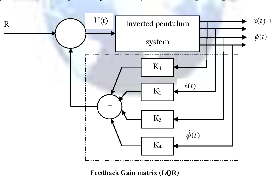
2. Intuition in Design: Poles vs. Weights
While pole placement seems direct, its intuition breaks down quickly as system complexity increases.
- For a simple second-order system, you know that placing poles further to the left in the complex plane results in a faster response.
- But what about a fourth-order system like the inverted pendulum, or a higher-order multivariable system? Where should you place the third and fourth poles? How does moving one pole affect the control effort required? The answers are far from obvious.
LQR offers a different, and often more intuitive, way to tune the system, especially for the multi-input, multi-output (MIMO) systems you're focusing on. Instead of thinking about abstract pole locations, you think about the physical behavior of the system.
The following video segment demonstrates this power of LQR tuning.
What Is Linear Quadratic Regulator (LQR) Optimal Control? | State Space, Part 4
This part of the MATLAB video shows a practical example of why tuning LQR can be more intuitive than pole placement, especially when dealing with physical constraints like actuator saturation.
Watch from 15:00 to 16:44. The presenter has a 3-state system where the initial controller requires too much actuator effort. Notice the question posed: 'had we developed this controller using pole placement, the question at this point would be which of these three poles should we move in order to reduce the actuator effort?' Then, see how easily this is solved in LQR by simply increasing the penalty in the R matrix.
The video makes a powerful point: with LQR, the tuning process is directly linked to performance objectives.
- Problem: "My actuator is saturating."
- LQR Solution: Increase the value in . This tells the controller to be more conservative with control effort.
- Problem: "The pendulum angle is not stabilizing fast enough."
- LQR Solution: Increase the corresponding diagonal element in . This tells the controller to prioritize reducing the error in that specific state.
This approach of tuning weights is generally more scalable and intuitive for complex, multivariable systems than trying to decide where to place a large number of poles.
3. Optimality and Robustness Guarantees
This is perhaps the most significant theoretical difference between the two methods.
Pole Placement provides a controller that meets your pole location criteria, but it offers no guarantee of optimality or robustness. It's possible to place poles for a very fast response, but this might result in a system that is very sensitive to small errors in your mathematical model (i.e., it has poor stability margins).
LQR, by contrast, is provably optimal for the cost function you define. More importantly from a practical standpoint, it comes with remarkable, built-in robustness guarantees. For a single-input system, an LQR controller is guaranteed to have:
- An infinite upward gain margin.
- A gain reduction margin of at least 50%.
- A phase margin of at least .
While the guarantees are more complex for MIMO systems, LQR is renowned for producing controllers with good stability margins. This means your controller is more likely to work on the real physical system, even if your model isn't perfect. This is a major advantage that pole placement does not provide.
Test your understanding!
You are tasked with designing a flight controller for a new, experimental quadcopter. The system has 12 states and 4 inputs. Your aerodynamic model is just an approximation, so you anticipate that the real-world dynamics will differ slightly from your simulation.
Which design method, Pole Placement or LQR, would be a more suitable starting point, and why?
Show answer
LQR would be the more suitable choice.
Here's the reasoning:
- Complexity: A 12-state system means you would need to intelligently choose 12 closed-loop pole locations for the pole placement method. This is a highly non-intuitive and difficult task. With LQR, you can start by tuning the 12 elements of the diagonal Q matrix and 4 elements of the R matrix based on physical priorities (e.g., "prioritize altitude stability," "conserve battery power").
- Robustness: Since the model is an approximation, robustness to uncertainty is critical. LQR's inherent stability margins provide a much safer starting point than pole placement, which offers no such guarantees. The LQR controller is more likely to be stable on the actual hardware.
4. Comparison on the Rotary Inverted Pendulum
Let's bring this comparison to the system you're interested in. The following research paper provides a direct comparison of the two techniques for stabilizing a rotary arm inverted pendulum.
Stabilization of Rotary Arm Inverted Pendulum using State Feedback Techniques
This paper, 'Stabilization of Rotary Arm Inverted Pendulum using State Feedback Techniques', directly implements and compares the two controllers we're discussing. Reading their design process and conclusions will provide a concrete example of the trade-offs.
Please read the following sections from the PDF: Section III.A 'Pole Placement Controller': Note how the authors choose the desired poles based on damping ratio and time constants. Section III.B 'LQR controller': See how they instead choose different sets of Q matrices to find a good response. Section IV 'SIMULATION RESULTS' and V 'CONCLUSION': Read the authors' analysis of the results. Pay attention to their final comparison regarding transient response, steady-state error, and ease of tuning.
The paper's conclusion highlights a common finding:
- They found pole placement was "better to improve the transient response." This is because they explicitly designed it for a specific transient response by choosing dominant poles.
- They found LQR was better for "minimizing the steady state value."
- Crucially, they note: "It is always not easy to obtain the gain matrix for state feedback [pole placement] controller easily. But in the case of LQR controller the gain matrix K can be tuned easily to obtain the desired response."
This last point echoes our discussion on intuition. While you can achieve a desired transient response with LQR by carefully tuning Q and R, the process is often more straightforward and less of a guessing game than picking a full set of poles for a complex system.
Conclusion: Which to Choose?
We can summarize the comparison in the following table:
| Feature | Pole Placement | Linear Quadratic Regulator (LQR) |
|---|---|---|
| Design Input | Desired closed-loop pole locations () | Weighting matrices for state and control effort () |
| Philosophy | "Place the poles here to get this response." | "Find the best controller that balances this performance cost." |
| Intuition | Good for low-order systems. Difficult for high-order/MIMO. | More intuitive for complex/MIMO systems via physical weights. |
| Optimality | Not optimal in any formal sense. | Provably optimal for the given cost function . |
| Robustness | No inherent guarantees. Can result in fragile designs. | Excellent guaranteed stability margins (e.g., phase margin). |
Key Takeaways:
- Both Pole Placement and LQR are state feedback techniques that calculate a gain matrix , but they do so based on fundamentally different design philosophies.
- Pole Placement gives you direct control over pole locations, which is powerful for simple systems but becomes highly unintuitive for complex, multivariable systems.
- LQR's approach of tuning weighting matrices ( and ) is often more intuitive, scalable, and directly related to physical performance goals (e.g., "reduce position error" or "save fuel").
- LQR provides proven optimality and, most importantly, excellent robustness guarantees, making it a safer and more reliable choice when dealing with model uncertainties. For multivariable control, LQR is very often the superior method.
Preview of the Next Module:
Congratulations on completing the LQR module! So far, all the controllers we have designed have been regulators—their primary job is to take a system from a disturbed state and return it to the zero-state equilibrium point.
However, in most real applications, we want our system to follow a specific command. We don't just want the inverted pendulum to stay balanced at ; we want to command it to move to meters and stay there. In the next module, we will build upon our state-feedback foundation to tackle reference tracking and disturbance rejection, two essential topics for creating practical, high-performance control systems.