Pole Placement for Performance

Hello! Welcome to the first lesson in our module on state feedback control.

In our previous lessons, we analyzed our system's structure. We learned how to model it, check for controllability, and use the Relative Gain Array (RGA) to understand how different inputs and outputs are coupled. This analysis was about understanding the problem we need to solve. Now, we shift our focus from analysis to design. We will start building a controller that makes the system behave the way we want it to.

Our first design technique is pole placement, a cornerstone of modern control theory. The central idea is to "place" the poles of our closed-loop system at specific locations in the complex plane to achieve a desired performance. But this begs the question: how do we choose where to put them?

This lesson will equip you with the knowledge to answer that question. We will focus on the learning outcome: Select desired closed-loop pole locations to meet performance specifications like settling time and damping. By the end of this lesson, you'll be able to translate intuitive performance goals like "be fast" or "don't overshoot" into the precise mathematical language of pole locations.

From Performance Goals to Time-Domain Specifications

When we design a control system, our goals are often expressed in plain language. For the rotary inverted pendulum, we might want it to "swing up quickly and stabilize with minimal wobble." For a drone's altitude controller, we want it to "reach the target height without overshooting and getting into a restricted airspace."

To design a controller, we must translate these qualitative goals into quantitative metrics. The most common way to do this is by analyzing the system's step response.

The Step Response | Control Systems in Practice

This video from MATLAB provides a clear introduction to the step response and the key performance metrics derived from it.

Please watch from the beginning to 4:16. Focus on the definitions of the four key metrics used to characterize a step response.

As the video explained, we can characterize the transient response of a system using these four key metrics:

Rise Time ( $t_{r}$ ): The time it takes for the response to go from 10% to 90% of its final value. This is a measure of speed.
Percent Overshoot (%OS): The maximum amount by which the response exceeds its final steady-state value, expressed as a percentage. This measures the tendency to oscillate.
Settling Time ( $t_{s}$ ): The time required for the response to enter and stay within a certain tolerance band (usually ±2% or ±5%) of its final value. This quantifies how long it takes for transients to die out.
Steady-State Error ( $e_{ss}$ ): The difference between the desired final value (the reference) and the actual final value of the response.

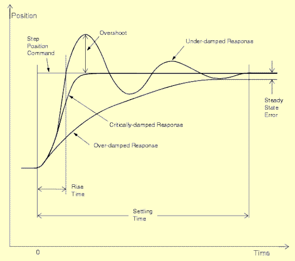
Step Response Characteristics of Control Systems — A typical step response showing key performance metrics. The under-damped response is often of most interest, as it exhibits a trade-off between speed and overshoot.

The Link to Second-Order Systems

For many systems, we can approximate their behavior using a standard second-order system model. Your background in electrical engineering will make this concept familiar; it's analogous to analyzing an RLC circuit. The beauty of this approach is that it reduces the four performance metrics we just discussed to just two fundamental parameters: the natural frequency ( $ω_{n}$ ) and the damping ratio ( $ζ$ ).

A canonical second-order system without zeros has the transfer function:

G (s) = \frac{ω _{n}^{2}}{s ^{2} + 2 ζ ω _{n} s + ω _{n}^{2}}

Damping Ratio ( $ζ$ ): This dimensionless parameter dictates the shape of the response, primarily the percent overshoot.
- $ζ = 0$ : Undamped (pure oscillation)
- $0 < ζ < 1$ : Underdamped (overshoots and oscillates)
- $ζ = 1$ : Critically damped (fastest response with no overshoot)
- $ζ > 1$ : Overdamped (slow, no overshoot)
Natural Frequency ( $ω_{n}$ ): This parameter dictates the speed of the response. A higher $ω_{n}$ "compresses" the response in time, leading to a faster rise time and settling time.

The following video segment provides an excellent visualization of how changing $ζ$ and $ω_{n}$ affects the step response.

The Step Response | Control Systems in Practice

Continuing with the same MATLAB video, this section visually demonstrates the relationship between natural frequency, damping ratio, and the time-domain response.

Watch from 10:52 to 14:32. Pay close attention to how adjusting the \zeta slider primarily changes the overshoot, while the \omega_n slider speeds up or slows down the entire response.

From Damping and Frequency to Pole Locations

Now we come to the core of the lesson: connecting these parameters to pole locations. The poles of a system are the roots of its characteristic equation (the denominator of the transfer function). For our standard second-order system, the poles are:

s = - ζ ω_{n} \pm ω_{n} ζ^{2} - 1

For the most common case of an underdamped system ( $0 < ζ < 1$ ), this is written as:

s = - ζ ω_{n} \pm j ω_{n} 1 - ζ^{2}

Here, $s = σ \pm j ω_{d}$ , where:

$σ = - ζ ω_{n}$ is the real part, determining the rate of exponential decay (related to settling time).
$ω_{d} = ω_{n} 1 - ζ^{2}$ is the imaginary part, known as the damped natural frequency, which sets the frequency of oscillations.

This relationship allows us to map desired performance onto the complex s-plane.

Second-Order Closed-Loop Pole Location and System Response — This diagram illustrates the relationship between pole locations in the s-plane and system response. Poles on circles of constant radius have the same natural frequency ($\omega_n$). Poles on rays from the origin have the same damping ratio ($\zeta$). Poles on the same vertical line share the same real part, $\sigma$, and thus have the same settling time.

To move from design specifications to pole locations, we use a set of well-known formulas.

Controller Design Using Pole Placement

This section from a lab manual by the University of Toronto provides the direct formulas needed to calculate the required \zeta and \omega_n from performance specifications.

Please read Section 2.1, 'Choosing the closed loop poles'. Focus on equations (4) and (5), which show how to find \zeta from percent overshoot (%OS) and \omega_n from peak time (t_p). Note that similar formulas exist relating these parameters to settling time (t_s).

Based on the resource, the key formulas are:

To find $ζ$ from a desired %OS:
$ζ = \frac{- l n ( % O S /100 )}{π ^{2} + l n ^{2} ( % O S /100 )}$
A common approximation for the 2% settling time is:
$t_{s} \approx \frac{4}{ζ ω _{n}}$
From this, we can find the required real part of the poles: $σ = - ζ ω_{n} \approx - 4/ t_{s}$ .

Once you have $ζ$ and $ω_{n}$ , you can calculate the desired pole locations $s = - ζ ω_{n} \pm j ω_{n} 1 - ζ^{2}$ .

Test your understanding!

You are designing a controller and have the following performance requirements for the closed-loop system:

Percent Overshoot (%OS) $\leq$ 5%
Settling time ( $t_{s}$ , 2% criterion) $\leq$ 2 seconds

Determine the desired locations for the dominant closed-loop poles.

Show answer

Find the damping ratio $ζ$ from the %OS requirement:
Using the formula for %OS = 5% (or 0.05):
$ζ = \frac{- ln ( 0.05 )}{π ^{2} + ln ^{2} ( 0.05 )} = \frac{2.9957}{9.8696 + ( 2.9957 ) ^{2}} = \frac{2.9957}{18.8438} \approx 0.69$
Find the product $ζ ω_{n}$ from the settling time requirement:
Using the 2% settling time approximation:
$t_{s} \approx \frac{4}{ζ ω _{n}} ⟹ ζ ω_{n} \approx \frac{4}{t _{s}} = \frac{4}{2} = 2$
So the real part of our poles should be at $σ = - 2$ .
Find the natural frequency $ω_{n}$ :
Since $ζ ω_{n} = 2$ and $ζ \approx 0.69$ :
$ω_{n} = \frac{2}{0.69} \approx 2.9 rad/s$
Calculate the pole locations:
The poles are at $s = - ζ ω_{n} \pm j ω_{n} 1 - ζ^{2}$ .
$s = - 2 \pm j (2.9) 1 - 0.6 9^{2} = - 2 \pm j (2.9) (0.7238) \approx - 2 \pm j 2.1$
Therefore, the desired closed-loop pole locations are approximately $s = - 2 \pm j 2.1$ .

Handling Higher-Order Systems: Dominant Poles

The inverted pendulum you are working on is a 4th-order system, not a simple 2nd-order one. So how do we apply these principles? The key is the concept of dominant poles.

In any system, the poles closest to the imaginary axis in the s-plane have the slowest decay rates and therefore dominate the transient response. Poles located much further to the left correspond to modes that decay very quickly and have a negligible effect on the overall system behavior after a short time.

The practical design strategy is:

Design the system to have a pair of complex-conjugate dominant poles at the locations calculated from your desired second-order performance ( $ζ$ and $ω_{n}$ ).
Place the remaining poles of the system significantly "faster" than the dominant pair—that is, much further to the left in the s-plane (e.g., 5 to 10 times the real part of the dominant poles). These can be real poles to avoid introducing additional oscillations.

What is Pole Placement (Full State Feedback) | State Space, Part 2

This short clip from a MATLAB video on pole placement introduces the concept of dominant poles for higher-order systems.

Watch from 12:47 to 13:16. It gives the main idea of placing two poles to dominate the response while noting the practical limits of actuators.

This strategy is exactly what is used in practice, including for the rotary inverted pendulum.

Rotary Inverted Pendulum Control Project

This resource, a project guide for a rotary inverted pendulum, shows a practical application of the dominant pole concept.

Read Section 2.2, 'Closed-loop poles specifications'. Notice how they specify a desired response using a dominant second-order pair (defined by a time constant au=1/(\zeta\omega_n) and damping ratio \zeta) and then select two other real, faster poles.

Conclusion

In this lesson, we have built the bridge between high-level performance goals and the specific, mathematical targets needed for controller design. You now have a systematic process for determining where your closed-loop poles should be located.

Key Takeaways:

Performance specifications like percent overshoot and settling time are used to quantify the desired behavior of a control system.
For a standard second-order system, these specs map directly to the damping ratio ( $ζ$ ) and natural frequency ( $ω_{n}$ ).
The values of $ζ$ and $ω_{n}$ define the location of the closed-loop poles in the complex s-plane: $s = - ζ ω_{n} \pm j ω_{n} 1 - ζ^{2}$ .
For higher-order systems, we use the dominant pole concept: we place a pair of poles to achieve the desired second-order response and place all other poles much further into the left-half plane so their transient effects are negligible.

Preview of the Next Lesson:
We have successfully defined our target. We know where we want our closed-loop poles to be. In the next lesson, we will learn the mechanics of pole placement: how to calculate the state feedback gain matrix, $K$ , that will take the system's original poles and move them to our desired locations.

Recommended resources

From Performance Goals to Time-Domain Specifications

The Link to Second-Order Systems

From Damping and Frequency to Pole Locations

Handling Higher-Order Systems: Dominant Poles

Conclusion