Visualizing Data with Matplotlib and Seaborn

1. Introducing Seaborn: Making Data Visualization Easier

Python has a powerful foundational plotting library called Matplotlib. While it can create almost any plot imaginable, the code can sometimes be verbose. Seaborn is another library built on top of Matplotlib. It's specifically designed for creating attractive and informative statistical graphics with much simpler code. For our purposes, we'll primarily use Seaborn.

Let's start by seeing how to set up your environment and load some data for plotting.

As you saw, the basic setup involves importing the libraries and loading a dataset into a Pandas DataFrame:

# The standard way to import these libraries
import seaborn as sns
import matplotlib.pyplot as plt

# Load a built-in dataset from Seaborn
tips = sns.load_dataset("tips")

# Display the first few rows to see what it looks like
print(tips.head())

2. Histograms: Visualizing a Variable's Distribution

Remember how we calculated the mean and standard deviation in the last lesson? A histogram lets you see that information. It shows the shape of your data's distribution, making it easy to spot if the data is symmetric (like a Normal distribution) or skewed.

A histogram works by grouping data into intervals or "bins" and then plotting the number of data points that fall into each bin.

Let's see how to create one.

As the video shows, creating a histogram is straightforward:

# Create a histogram of the 'total_bill' column
sns.histplot(data=tips, x="total_bill", bins=20, kde=True)
plt.show() # This command displays the plot

How to Interpret a Histogram:

• X-axis: Shows the values of the variable (e.g., total bill amount).
• Y-axis: Shows the frequency (count) of observations within each bin.
• Shape: Look at the overall shape. Is it tall in the middle and short on the sides (symmetric)? Or is there a long "tail" to one side (skewed)? In our total_bill example, we can see a "right skew," meaning most bills are on the lower end, with a few very high bills pulling the tail to the right.

3. Scatter Plots: Visualizing Relationships Between Two Variables

What if you want to know if two variables are related? For example, do people with higher total bills also leave higher tips? A scatter plot is the perfect tool for this. It places a dot for each data point on a 2D graph, with one variable on the x-axis and another on the y-axis.

How to Interpret a Scatter Plot:

• Positive Correlation: If the dots generally trend upwards from left to right, it indicates a positive relationship (as one variable increases, the other tends to increase). You can see this clearly in the total_bill vs. tip plot.
• Negative Correlation: If the dots trend downwards from left to right, it's a negative relationship.
• No Correlation: If the dots are scattered randomly with no clear trend, there is likely no relationship.

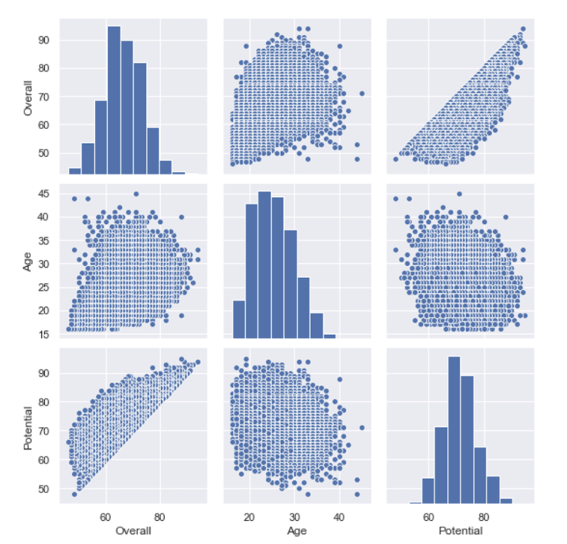
A common and powerful way to quickly view the distributions and pairwise relationships of multiple variables is with a pair plot.

4. Box Plots: Summarizing Distributions and Finding Outliers

In the last lesson, you used .describe() to get a five-number summary (min, 25%, 50%, 75%, max). A box plot (or box-and-whisker plot) is a visual representation of that exact summary. It's incredibly useful for seeing a variable's spread and identifying potential outliers.

Before we create one, let's understand its components.

This image perfectly illustrates how the shape of a histogram relates to the resulting box plot.

Now, let's see how to create and use box plots, especially for comparing distributions across different categories.

A common use case for a box plot is to compare a numerical variable across different groups of a categorical variable. For example, let's compare the distribution of total_bill for each day of the week.

# Create a box plot to compare total_bill across different days
sns.boxplot(data=tips, x="day", y="total_bill")
plt.title("Distribution of Total Bill by Day")
plt.show()

From this single plot, you can immediately compare the median bill, the range of typical bills (the box), and the presence of outliers for each day.

Conclusion

Fantastic work today! You have now moved from calculating statistics to visualizing them, a critical skill for anyone working with data. Visualizations make complex data intuitive and are your best friends during exploratory analysis.

Key Takeaways:

• Seaborn is a high-level library that simplifies the creation of statistical plots.
• Histograms are used to understand the distribution (shape, center, spread) of a single numerical variable.
• Scatter Plots are used to investigate the relationship or correlation between two numerical variables.
• Box Plots provide a five-number summary of a numerical variable, are excellent for identifying outliers, and are ideal for comparing distributions across different categories.

Preview of the Next Lesson:

You've now completed the module on Probability and Statistics! We've covered a lot, from theoretical distributions to practical data analysis with Pandas and Seaborn.

In the next module, we will switch gears and dive into Core Data Structures. The first lesson will be on analyzing algorithm efficiency using Big-O notation. As you start to write code to process and analyze data, it becomes crucial to understand how efficient that code is, especially when dealing with large datasets. Big-O notation is the language we use to describe that efficiency.