Bias, Variance, Underfitting, and Overfitting

1. A Picture of Prediction Errors: The Dartboard Analogy

Before we get into formal definitions, let's start with a simple analogy. Imagine you're throwing darts at a dartboard. The bullseye represents the true, correct value you want your model to predict. Each dart you throw is one prediction.

Let's break down the four scenarios shown in the image:

• Low Bias, Low Variance (Top-Left): Your darts are tightly clustered right at the bullseye. This is the ideal scenario. Your predictions are accurate and consistent.
• High Bias, Low Variance (Bottom-Left): Your darts are tightly clustered, but they consistently miss the bullseye in the same spot. Your model has a systematic error, but it's consistent.
• Low Bias, High Variance (Top-Right): Your darts are scattered all over the board, but their average position is the bullseye. Your model is correct on average, but individual predictions are unreliable and inconsistent.
• High Bias, High Variance (Bottom-Right): Your darts are scattered all over the board, and they are not even centered on the bullseye. This is the worst-case scenario. Your predictions are both inaccurate and inconsistent.

This analogy gives us a great starting point for understanding the two main sources of reducible error in machine learning: bias and variance.

2. Understanding Bias and Underfitting

Bias is the error introduced by a model's simplifying assumptions. If a model is too simple, it can't capture the true, complex patterns in the data. This leads to high bias.

Think of trying to fit a straight line to data that has a curved relationship. No matter how you adjust the line, it will never be able to capture the curve. This inability to model the true relationship is bias.

A model with high bias is said to underfit the data.

• Symptom: An underfitting model performs poorly on the training data and also performs poorly on the test data. Its errors are high everywhere because it's simply not a good model for the data.

This first video gives a fantastic visual explanation of bias.

3. Understanding Variance and Overfitting

Variance is the error introduced because a model is overly sensitive to the specific data it was trained on. A model that is too complex might learn not just the underlying patterns (the "signal") but also the random fluctuations and noise in the training data. This leads to high variance.

This model might look perfect on the training data, but because it has essentially memorized the noise, it won't generalize well to new, unseen data.

A model with high variance is said to overfit the data.

• Symptom: An overfitting model performs exceptionally well on the training data (very low error) but performs poorly on the test data (high error). This large gap between training and test performance is the classic sign of overfitting.

Let's continue with the StatQuest video to see what high variance looks like.

4. Diagnosing Underfitting and Overfitting

We can diagnose these issues by comparing the model's error on the training set versus the test set. The next video walks through a great example using polynomial regression, where increasing the model's complexity (the degree of the polynomial) takes us from underfitting to a good fit, and finally to overfitting.

This leads us to a simple, practical guide for diagnosis, which is also summarized well in the "Bias-Variance Tradeoff, Explained" article.

5. The Bias-Variance Tradeoff

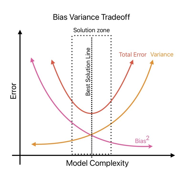
As you might have guessed, bias and variance are in a constant tug-of-war. This relationship is known as the Bias-Variance Tradeoff.

• Simple Models (like linear regression) tend to have high bias and low variance. They are stable but often inaccurate.
• Complex Models (like a high-degree polynomial or a deep decision tree) tend to have low bias and high variance. They are flexible and can be accurate, but they are also unstable and prone to overfitting.

Our goal as data scientists is not to eliminate bias or variance entirely, but to find a "sweet spot" in model complexity that minimizes the total error.

Decomposing the Total Error

Mathematically, the total expected error of a model (specifically, the Mean Squared Error) can be broken down into three components:

$\text{Total Error}={\text{Bias}}^2+\text{Variance}+\text{Irreducible Error}$

We've discussed bias and variance. But what is Irreducible Error?

It's the inherent randomness or "noise" in a dataset that cannot be predicted by any model, no matter how perfect. It comes from factors that are not measured or are fundamentally unpredictable (like random human behavior in a house sale). This error sets the ultimate limit on how well any model can perform.

Conclusion

In this lesson, you've learned about the fundamental sources of error in machine learning models. This is a critical diagnostic skill for building effective models and a frequent topic in exams like GATE.

Key Takeaways:

• Bias is error from a model being too simple (underfitting). It's diagnosed by high error on both training and test data.
• Variance is error from a model being too complex and sensitive to noise (overfitting). It's diagnosed by a large gap between low training error and high test error.
• The Bias-Variance Tradeoff describes the inverse relationship between bias and variance as model complexity changes.
• The goal of model tuning is to find the optimal complexity that minimizes the sum of bias and variance, achieving the lowest possible total error on unseen data.
• Irreducible Error is the baseline noise in the data that no model can eliminate.

Preview of the Next Lesson:
Now that we can diagnose overfitting, what can we do about it? In our next lesson, we will explore powerful techniques called L1 (Lasso) and L2 (Ridge) regularization, which are specifically designed to combat overfitting by penalizing model complexity.