CNN Architecture for Image Data

1. Why Not Just Use a Bigger FNN?

In the previous lesson, we flattened our 28x28 pixel images into a 784-element vector to feed into our fully connected network. This approach has two major problems when dealing with images:

1. Loss of Spatial Information: An image isn't just a random collection of pixels; it has spatial structure. Neighboring pixels are highly related. By flattening the image, we throw away this crucial information. The network has no inherent knowledge that pixels in the top-left corner are far from pixels in the bottom-right.
2. Parameter Explosion: Our simple 28x28 grayscale images were manageable. But consider a more standard 224x224 color image. This would mean 224 * 224 * 3 = 150,528 input neurons. A single hidden layer with 1000 neurons would require over 150 million weights! This is computationally infeasible to train and extremely prone to overfitting.

To address these issues, we need an architecture that respects the spatial structure of images and is more efficient with its parameters. This is where Convolutional Neural Networks come in.

2. The Building Blocks of a CNN

A CNN is built from a few key layers that are stacked together. A typical CNN architecture consists of two main parts: a Feature Extraction part and a Classification part.

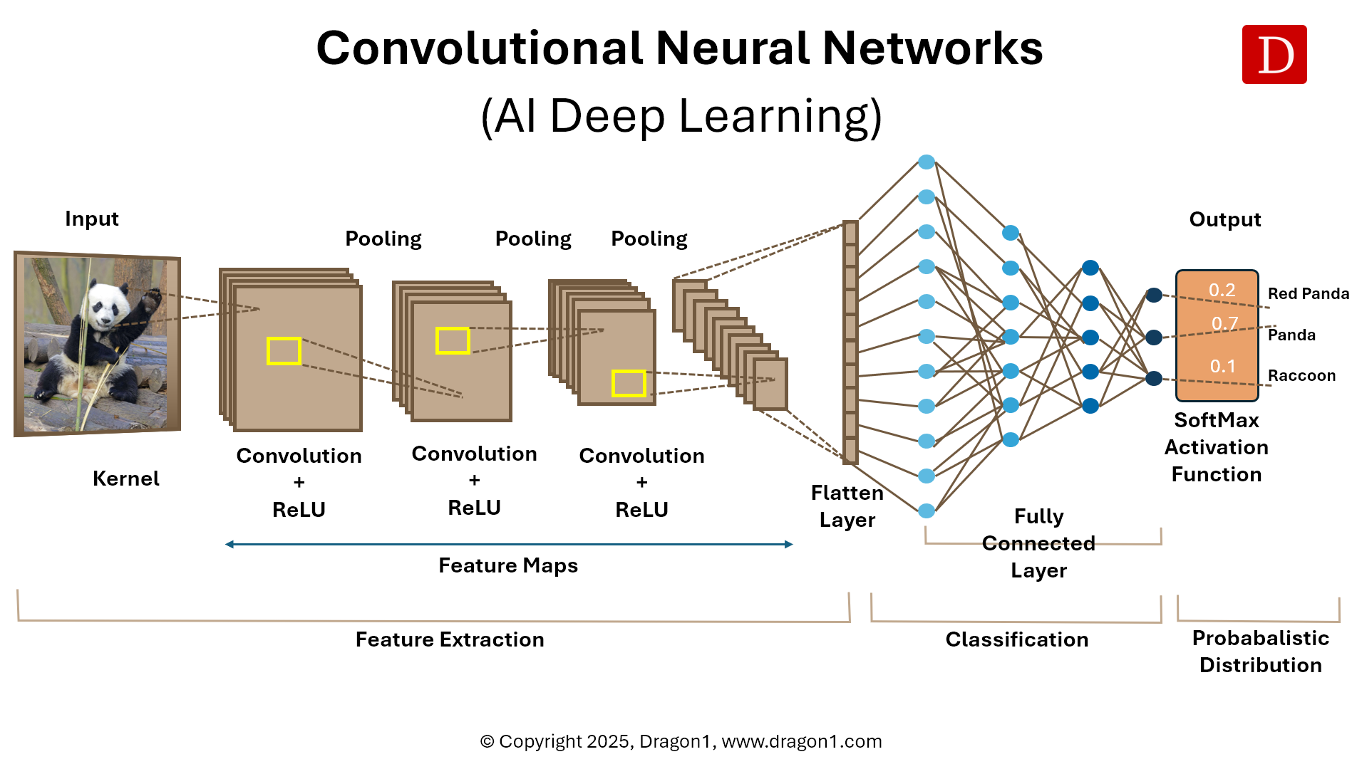
Let's break down the "ingredients" used to build these stages.

Ingredient 1: The Convolutional Layer

The core of a CNN is the convolutional layer. Instead of connecting every input to every neuron, this layer uses a small grid of weights called a filter (or kernel) that slides over the input image.

• The Operation: At each position, the filter performs an element-wise multiplication with the patch of the image it's currently covering and then sums up the results into a single output pixel. This sliding operation is called a convolution.
• Feature Detection: Each filter learns to recognize a specific low-level feature, such as a vertical edge, a horizontal edge, a specific color, or a corner. By using multiple filters in a single layer, the network can learn to detect many different features simultaneously.
• The Output: The output of this operation is called a feature map or activation map. It's a 2D grid that shows where the filter detected its specific feature in the input image.

This process is explained very clearly in the next segment of the StatQuest video.

The key ideas here are local connectivity (each neuron in the feature map is connected to only a small patch of the input) and parameter sharing (the same filter is used across the entire image), which dramatically reduces the number of parameters.

To get a more detailed look, this next video from MIT's Deep Learning course provides an excellent, intuitive explanation of how filters are used to detect patterns.

Key Parameters of a Convolutional Layer:
When we define a convolutional layer in PyTorch, we'll see a few important parameters.

• kernel_size: The dimensions of the filter (e.g., 3x3, 5x5).
• stride: The number of pixels the filter "steps" or "slides" at a time. A stride of 1 means it moves one pixel at a time.
• padding: Adding a border of zeros around the image. This allows the filter to process the edges of the image properly and can help control the output size of the feature map.
• out_channels: The number of filters to use in the layer. This determines the number of feature maps the layer will produce.

Ingredient 2: The Activation Function (ReLU)

Just as with FNNs, after each convolution, we apply a non-linear activation function. The most common choice in CNNs is the Rectified Linear Unit (ReLU). It is applied element-wise to the feature map, setting all negative values to zero. This introduces non-linearity, allowing the network to learn more complex patterns.

Ingredient 3: The Pooling Layer

After the activation function, we often add a pooling layer. Its primary purpose is to downsample the feature maps, reducing their spatial dimensions (width and height).

• How it Works: It operates over a small window (e.g., 2x2) and reduces the values in that window to a single value. The most common method is Max Pooling, which simply takes the maximum value from the window.
• Benefits:
  1. Reduces Computation: Smaller feature maps mean fewer parameters and less computation in later layers.
  2. Creates Local Invariance: It makes the feature detection more robust. If a feature is detected anywhere within the pooling window, the output will be similar. This means the network is less sensitive to the exact position of features.

Ingredient 4: The Fully Connected Layer (Classifier)

After several rounds of Convolution -> ReLU -> Pooling, the network has generated high-level feature maps that represent the content of the image. The Feature Extraction phase is complete.

Now, for the Classification phase:

1. The final 2D feature maps are flattened into a single 1D vector.
2. This vector is fed into a standard fully connected network (just like the one you built in previous lessons) which acts as a classifier.
3. The final layer of this FNN outputs the scores for each class (e.g., 10 scores for the digits 0-9).

This final part of the process connects the learned features to the final classification task.

3. Hierarchical Feature Learning

A powerful property of deep CNNs is that they learn features in a hierarchical manner.

• Early Layers (close to the input image) learn to detect very simple features like edges, corners, and color gradients.
• Deeper Layers receive their input from the feature maps of earlier layers. They learn to combine these simple features into more complex ones, like eyes, noses, or ears.
• Final Layers combine these complex features to recognize entire objects, like faces or cars.

Impressively, the network learns this entire hierarchy automatically from the data during training!

Conclusion

In this lesson, you've learned about the fundamental architecture of Convolutional Neural Networks. We moved from the limitations of fully connected networks to a new design that is far more effective and efficient for image data.

Key Takeaways:

• Why CNNs?: They solve the problems of FNNs for images by preserving spatial structure and being parameter-efficient.
• Convolutional Layers: Use learnable filters (kernels) to scan for features, creating feature maps. This is the core of feature extraction.
• Activation (ReLU): Introduces non-linearity, allowing the model to learn complex relationships.
• Pooling Layers (Max Pooling): Downsample feature maps to reduce computational cost and provide local invariance.
• Fully Connected Layers: Act as a classifier at the end of the network, taking the learned features as input to make a final prediction.
• Hierarchical Features: CNNs automatically learn a hierarchy of features, from simple edges in early layers to complex objects in deeper layers.

Preview of the Next Lesson:
Theory is great, but practice is better. Now that you understand the blueprint of a CNN, our next lesson, "Build and train a simple CNN for an image classification task," will guide you through implementing this architecture in PyTorch. You'll use nn.Conv2d and nn.MaxPool2d to build your own CNN and then plug it into the training loop you've already mastered to classify MNIST digits with even higher accuracy.