Hello! Welcome to your next lesson in the "Deep Learning with PyTorch" module.
In our previous lesson, you successfully built and trained a Convolutional Neural Network (CNN) to recognize handwritten digits. You saw how CNNs are architecturally designed to handle spatial data like images, using concepts like convolutional and pooling layers.
However, many of the most exciting problems in AI don't involve static images, but rather sequences of data where order is critical. Think about translating a sentence, predicting stock prices, or generating music. In these cases, the model needs a form of "memory" to understand context.
Today, we will dive into the architectures designed specifically for this purpose. Our learning goal is to describe the architecture of Recurrent Neural Networks (RNNs) and their powerful variant, Long Short-Term Memory (LSTM) networks. We will focus on the conceptual structure of these networks—how they are built and why their design allows them to process sequential data effectively.
Let's begin our exploration of networks that can remember the past.
1. What Are Recurrent Neural Networks (RNNs)?
Traditional neural networks, and even the CNNs you've worked with, process inputs independently. If you feed a CNN two different images, its analysis of the second image doesn't depend on what it saw in the first.
But what if you're reading a sentence? The meaning of each word depends heavily on the words that came before it. This is an example of sequential data. RNNs are designed to handle this by incorporating a loop, which allows information to persist from one step to the next. This persistent information is called the hidden state, and it acts as the network's memory.

To get a clear picture of how this works, let's watch a short video.
The Power of Recurrent Neural Networks (RNN)
This video from IBM Technology provides a great introduction to the fundamental concepts of RNNs.
Watch from the beginning to 03:24. Focus on: What makes RNNs different from regular neural networks. The concept of a 'loop' and 'memory'. The role of the hidden state ($h_t$) and how it's calculated using the current input ($x_t$) and the previous hidden state ($h_{t-1}$).
As you saw, the hidden state at each timestep is a function of both the current input and the previous hidden state . This simple recurrence relation is the key that allows RNNs to process sequences.
RNN Architectures for Different Tasks
This basic RNN unit can be arranged in various configurations to solve different problems, depending on the nature of the input and the desired output.
The Power of Recurrent Neural Networks (RNN)
RNNs are versatile. This next part of the video explains the common architectures and the tasks they are suited for.
Continue watching from 03:24 to 05:43. Try to link each architecture to a real-world application: Sequence-to-Vector: Sentiment analysis (classifying a whole movie review). Vector-to-Sequence: Image captioning (generating a sentence from an image). Encoder-Decoder (Seq-to-Vec-to-Seq): Language translation. Sequence-to-Sequence: Video classification on a frame-by-frame basis.
2. The Challenge: Long-Term Dependencies
In theory, RNNs can connect information across long sequences. For example, in the text "I grew up in France... I speak fluent French", the network should be able to connect "France" at the beginning to predict "French" at the end.
In practice, standard RNNs struggle with this. As the sequence gets longer, it becomes difficult for the network to carry relevant information from earlier steps. This is known as the long-term dependency problem. It arises from a technical issue during training called the vanishing or exploding gradient problem, where the signals used to update the network's weights either shrink to nothing or grow uncontrollably.
The Power of Recurrent Neural Networks (RNN)
This final clip from the IBM video introduces this critical challenge, which motivates the need for more advanced architectures.
Watch from 05:43 to 06:41. The goal here is not to understand the deep mathematics of gradients yet, but to grasp the conceptual problem: a simple RNN's 'memory' is often too short.
3. Long Short-Term Memory (LSTM) Networks
To address the long-term dependency problem, Long Short-Term Memory (LSTM) networks were developed. LSTMs are a special kind of RNN, explicitly designed to remember information for long periods.
Let's start our dive into LSTMs with a reading from a classic blog post that provides a superb conceptual overview.
This article by Christopher Olah is one of the most famous resources for understanding LSTMs. It provides clear explanations and excellent diagrams.
Read the first three sections: 'Recurrent Neural Networks', 'The Problem of Long-Term Dependencies', and 'LSTM Networks'. Focus on the visual comparison between the simple repeating module in a standard RNN and the more complex four-layered module in an LSTM.
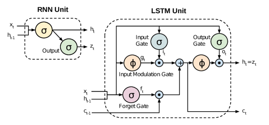
As the article illustrates, the key difference in an LSTM is its more complex repeating unit. This unit introduces a new component called the cell state, along with three "gates" that control the flow of information.
Core Components of an LSTM
- Cell State: Think of this as the network's long-term memory. It runs straight through the entire chain of repeating units, like a conveyor belt. Information can be added to or removed from the cell state, but it can also flow along it unchanged, which is crucial for preserving long-term information.
- Gates: These are structures that regulate the flow of information into and out of the cell state. They are essentially small neural networks with a sigmoid activation function, which outputs a value between 0 (let nothing through) and 1 (let everything through).
To see how these components work together, let's watch a detailed video walkthrough.
Long Short-Term Memory (LSTM), Clearly Explained
The video from StatQuest with Josh Starmer is famous for its clear, step-by-step explanations. It breaks down the complex LSTM unit into understandable parts.
Watch from the beginning to 06:46. Pay close attention to: The recap of the vanishing/exploding gradient problem. The core idea: an LSTM has separate paths for long-term memory (the cell state) and short-term memory (the hidden state). The identification of these two paths in the LSTM diagram.
The Three Gates: Forget, Input, and Output
The true power of the LSTM lies in its three gates, which learn to selectively remember, forget, and output information.
- Forget Gate: Decides what information to discard from the cell state. It looks at the previous hidden state () and the current input () and outputs a number between 0 and 1 for each piece of information in the previous cell state ().
- Input Gate: Decides what new information to store in the cell state. This is a two-part process:
- A sigmoid layer (the "input gate layer") decides which values to update.
- A
tanhlayer creates a vector of new candidate values that could be added to the state.
- Output Gate: Decides what the next hidden state should be. The hidden state is a filtered version of the cell state. The output gate uses a sigmoid to decide which parts of the cell state to output, which are then passed through a
tanhfunction.
Now that you have a conceptual overview, let's revisit the Colah blog post for a more detailed, diagram-based walkthrough of this process.
With the video's explanation in mind, this text-based walkthrough will help solidify your understanding of the gates. The diagrams are particularly insightful.
Read the sections 'The Core Idea Behind LSTMs' and 'Step-by-Step LSTM Walk Through'. For each step (forget, input, update, output), try to connect the explanation and the diagram to the concepts from the StatQuest video.
Test your understanding!
Imagine an LSTM is processing the sentence: "The cats are on the mat. They are sleeping."
When the model processes the word "They", what do you think the forget gate should ideally do with the "plural" information from "cats" that is stored in the cell state?
Show answer
When processing "They", the model needs to know that the subject is plural to correctly predict "are" instead of "is". Therefore, the forget gate should output a value close to 1 for the part of the cell state storing the "plural" information from "cats". This tells the network to keep this crucial piece of long-term information, even though several words have passed.
Visual Summary: RNN vs. LSTM
The added complexity of the LSTM is what gives it its power.
Conclusion
In this lesson, you've explored the fundamental architectures for processing sequential data.
Key Takeaways:
- Recurrent Neural Networks (RNNs) are designed for sequential data, using a hidden state as a form of memory that is passed from one timestep to the next.
- Standard RNNs struggle with the long-term dependency problem due to vanishing and exploding gradients, limiting their effective memory span.
- Long Short-Term Memory (LSTM) networks solve this problem with a more sophisticated architecture.
- LSTMs introduce a cell state for long-term memory and use three gates—forget, input, and output—to meticulously control the flow of information, allowing them to remember or forget things over long sequences.
Preview of the Next Lesson:
We have now described the architecture of these powerful networks. The next logical question is: How do they learn? In the next lesson, we will delve into the training process for RNNs, focusing on the backpropagation through time (BPTT) algorithm and its implications.