Hello! Let's dive into the next lesson in our module on "Algorithms: Sorting, Searching, and Design."
Introduction
In our last lesson, we explored simple sorting algorithms like Bubble Sort and Insertion Sort. You learned that while they are easy to implement, their average time complexity of makes them inefficient for large datasets. This is a significant bottleneck in real-world applications and competitive programming.
Today, we will tackle this problem head-on by exploring two of the most powerful and widely used sorting algorithms in computer science. These algorithms employ a clever strategy called "divide and conquer" to achieve significantly better performance.
Your learning outcome for this lesson is to: Implement and analyze advanced sorting algorithms: merge sort and quick sort.
By the end of this lesson, you will understand:
- The "divide and conquer" paradigm.
- The logic, implementation, and analysis of Merge Sort.
- The logic, implementation, and analysis of Quick Sort.
- The critical trade-offs between these two algorithms in terms of time, space, and stability.
This topic is a cornerstone of algorithm design and is frequently tested in the GATE exam. Let's begin with Merge Sort.
1. Merge Sort: The "Divide and Merge" Strategy
Merge Sort follows a simple but powerful principle:
- Divide: Recursively split the array into two halves until you have arrays containing just one element. A single-element array is, by definition, already sorted.
- Conquer (Merge): Merge the smaller sorted arrays back together in the correct order until you are left with a single, fully sorted array.
This systematic process of breaking down the problem and then combining the solutions is the essence of the "divide and conquer" approach.
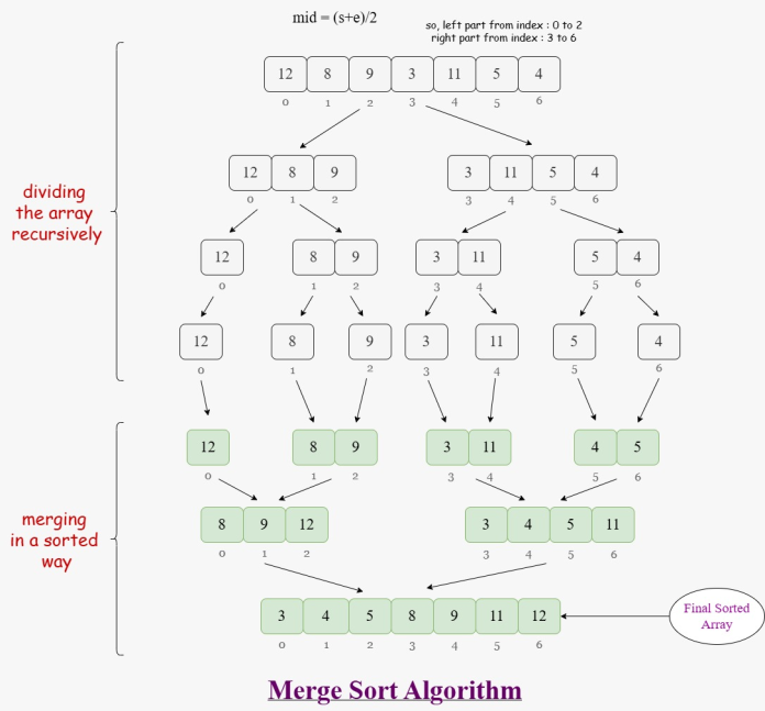
To see how this process works in detail, let's watch an excellent visual explanation.
Merge Sort | Algorithm | Pseudocode | Dry Run | Code | Strivers A2Z DSA Course
The video 'Merge Sort | Algorithm' from the 'take U forward' channel provides a fantastic step-by-step walkthrough of the divide and merge process. Pay close attention to how the array is hypothetically split and then pieced back together.
Watch from 01:11 to 13:39. This section explains the core logic of Merge Sort using a clear example. Focus on understanding the recursive division and the merging logic.
The merge Helper Function
As you saw in the video, the real work happens in the merge step. This step takes two already sorted sub-arrays and combines them into one larger sorted array. This is typically done by using two pointers, one for each sub-array, and comparing the elements to build the new sorted array.
Python Implementation
Implementing Merge Sort in Python involves creating two functions:
merge_sort(arr): The main function that handles the recursive division.merge(left, right): A helper function that merges two sorted lists.
Let's look at a clear and well-explained Python implementation.
Implementing the Merge Sort Algorithm in Python
This article from Codecademy, 'Implementing the Merge Sort Algorithm in Python', provides a clean Python implementation and breaks down the code for both the merge_sort and merge functions.
Read the section 'Merge sort implementation in python'. Study the code blocks for both merge_sort() and merge() to understand how the logic we just discussed is translated into code.
Here is the Python code from the article for your reference:
# The main recursive function
def merge_sort(arr):
    # Base case: A list with 0 or 1 element is already sorted.
    if len(arr) <= 1:
        return arr

    # 1. Divide
    mid = len(arr) // 2
    left_half = arr[:mid]
    right_half = arr[mid:]

    # Recursively sort both halves
    left_half = merge_sort(left_half)
    right_half = merge_sort(right_half)

    # 2. Conquer (Merge)
    return merge(left_half, right_half)

# The helper function to merge two sorted lists
def merge(left, right):
    result = []
    i = 0  # Pointer for the left list
    j = 0  # Pointer for the right list

    # Compare elements from both lists and add the smaller one
    while i < len(left) and j < len(right):
        if left[i] <= right[j]:
            result.append(left[i])
            i += 1
        else:
            result.append(right[j])
            j += 1

    # Append any remaining elements from the left or right list
    result.extend(left[i:])
    result.extend(right[j:])

    return result

# --- Example Usage ---
my_list = [38, 27, 43, 3, 9, 82, 10]
print(f"Unsorted Array: {my_list}")
sorted_list = merge_sort(my_list)
print(f"Sorted Array:   {sorted_list}")
Analysis of Merge Sort
Understanding the efficiency of Merge Sort is crucial for your GATE preparation.
-
Time Complexity:
- The
log npart comes from the number of times we can recursively divide the array in half. For an array of size , this happens approximately times. - The
npart comes from themergestep. At each level of recursion, we are merging a total ofnelements. - Crucially, Merge Sort's time complexity is in the best, average, and worst cases. This makes it very predictable and reliable.
- The
-
Space Complexity:
- During the
mergestep, we create a temporary array (resultin the code above) to store the merged elements. In the worst case, this temporary array will hold allnelements. This is a key disadvantage of Merge Sort, as it requires extra memory proportional to the input size.
- During the
For a deeper dive into the complexity analysis, you can review this section of the video.
Merge Sort | Algorithm | Pseudocode | Dry Run | Code | Strivers A2Z DSA Course
Let's revisit the 'take U forward' video to see the analysis of time and space complexity.
Watch the final segment from 44:18 to 47:30. This part explains where the 'n' and 'log n' components of the time complexity come from and discusses the O(n) space complexity.
Test your understanding!
Given the array [8, 4, 3, 7], what are the two sub-arrays that are passed to the merge function for the very first time in the merge_sort algorithm?
Show answer
The algorithm first divides the array completely.
[8, 4, 3, 7]is split into[8, 4]and[3, 7].- The left half
[8, 4]is split into[8]and[4].
These are single-element arrays (the base case), so they are returned.
The first merge operation will be on[8]and[4]. So, these are the first two sub-arrays passed to themergefunction. The result of this merge will be[4, 8].
2. Quick Sort: The "Partitioning" Strategy
Quick Sort is another highly efficient "divide and conquer" algorithm. However, its approach is different from Merge Sort.
- Divide (Partition): Select an element from the array, called the pivot. Rearrange the array so that all elements smaller than the pivot are placed before it, and all elements greater than the pivot are placed after it. After this partitioning, the pivot is in its final sorted position.
- Conquer: Recursively apply the same process to the two sub-arrays of elements (one with smaller values, one with larger values).
The key step is the partitioning. Unlike Merge Sort, where the main work is in combining (merging), Quick Sort does its main work in dividing (partitioning).

Let's watch a video that explains this pivot-and-partition strategy.
Quick Sort For Beginners | Strivers A2Z DSA Course
The video 'Quick Sort For Beginners' from the same 'take U forward' channel explains the core idea of picking a pivot and partitioning the array around it.
Watch from 01:01 to 17:30. This part covers the high-level explanation (01:01 - 13:08) and then delves into the pseudo-code logic of how the partitioning is actually performed using pointers (13:08 - 17:30). This is the most crucial part of the algorithm.
Python Implementation
The implementation of Quick Sort involves a main quick_sort function that calls a partition helper function.
QuickSort (With Code in Python/C++/Java/C)
The article 'Quicksort Algorithm' on Programiz provides a great explanation and a clear Python implementation of the algorithm. It shows how to implement the partition function which is the core of Quick Sort.
Scroll down to the 'Quicksort Code in Python, Java, and C/C++' section and study the Python code. Notice how the partition function rearranges the array and returns the final index of the pivot.
Here is the Python code from the article for your reference:
# Function to find the partition position
def partition(array, low, high):
    # Choose the rightmost element as pivot
    pivot = array[high]

    # Pointer for the greater element
    i = low - 1

    # Traverse through all elements and compare each with the pivot
    for j in range(low, high):
        if array[j] <= pivot:
            # If element smaller than pivot is found, swap it with the
            # greater element pointed to by i
            i = i + 1
            (array[i], array[j]) = (array[j], array[i])

    # Swap the pivot element with the element at the position after the last smaller element
    (array[i + 1], array[high]) = (array[high], array[i + 1])

    # Return the position where the partition is done
    return i + 1

# Main quick sort function
def quick_sort(array, low, high):
    if low < high:
        # Find pivot element such that elements smaller than pivot are on the left
        # and elements greater than pivot are on the right
        pi = partition(array, low, high)

        # Recursive call on the left of pivot
        quick_sort(array, low, pi - 1)

        # Recursive call on the right of pivot
        quick_sort(array, pi + 1, high)

# --- Example Usage ---
data = [8, 7, 2, 1, 0, 9, 6]
print(f"Unsorted Array: {data}")
size = len(data)
quick_sort(data, 0, size - 1)
print(f"Sorted Array:   {data}")
Analysis of Quick Sort
Quick Sort's performance analysis is more nuanced than Merge Sort's.
-
Time Complexity:
- Best and Average Case: . This occurs when the pivot selection consistently divides the array into roughly equal halves.
- Worst Case: . This is a critical point. The worst case happens when the pivot selection consistently produces highly unbalanced partitions. For example, if the pivot is always the smallest or largest element (which can happen if the array is already sorted and you always pick the first or last element as the pivot). This reduces the problem size by only one element at each step, leading to quadratic time complexity.
-
Space Complexity:
- Quick Sort is an in-place sorting algorithm. It does not require an auxiliary array like Merge Sort.
- The space it uses is on the recursion call stack. In the average case (balanced partitions), the recursion depth is . In the worst case (unbalanced partitions), it can be .
3. Merge Sort vs. Quick Sort: A Comparison
Choosing between Merge Sort and Quick Sort depends on the specific requirements of your problem. Here's a summary of their trade-offs:
| Feature | Merge Sort | Quick Sort |
|---|---|---|
| Time Complexity | in all cases (Best, Avg, Worst) | on average, but in the worst case |
| Space Complexity | (requires an auxiliary array) | (in-place, uses recursion stack space) |
| Stability | Stable | Not Stable |
| In Practice | More consistent performance. | Often faster on average due to better cache locality and being in-place. |
Stability is an important concept: a stable sorting algorithm maintains the original relative order of equal elements. For example, if you sort a list of students by grade, and two students have the same grade, a stable sort will keep them in their original alphabetical order. Merge Sort is stable, while Quick Sort is not.
Conclusion
You have now explored two of the most important sorting algorithms in computer science. They represent a major leap in efficiency over the simple algorithms.
Key Takeaways:
- Divide and Conquer is a powerful algorithmic paradigm that solves problems by breaking them into smaller, independent subproblems, solving them recursively, and combining their solutions.
- Merge Sort guarantees performance and is a stable sort, but at the cost of extra space.
- Quick Sort is typically faster in practice and is an in-place sort with space complexity, but its performance can degrade to in the worst case if the pivot is chosen poorly.
- Understanding the trade-offs between algorithms is a key skill for a data scientist and for the GATE exam.
Preview of the Next Lesson:
We've now covered two major algorithmic categories: searching and sorting. Next, we will venture into another powerful and fundamental algorithmic design paradigm: Dynamic Programming (DP). We will start by describing its core principles—optimal substructure and overlapping subproblems—which allow us to solve complex problems by breaking them down and storing the results of subproblems to avoid redundant calculations.