Hello! Welcome to the first lesson in our new module, "Algorithms: Sorting, Searching, and Design."
In the previous module, we focused on building core data structures like arrays, linked lists, hash tables, and heaps. We learned how to organize data efficiently. Now, we'll shift our focus to algorithms: the step-by-step procedures that operate on these data structures to solve specific problems.
This lesson tackles one of the most fundamental problems in computer science: searching. Imagine you have a massive dataset and you need to find one specific piece of information. How would you do it? Today, we will explore two classic approaches to this problem.
Your learning outcome for this lesson is to: Implement linear search and binary search algorithms and analyze their complexities.
We will cover:
- The concept and Python implementation of Linear Search.
- The concept and Python implementation of Binary Search.
- How to analyze the efficiency of these algorithms using Big-O notation (time complexity).
- The trade-offs between these two methods and why this is a key topic for your GATE exam preparation.
Let's begin with the most straightforward approach.
1. Linear Search: The Sequential Approach
Linear search, also known as sequential search, is the most intuitive searching algorithm. It works just like you'd expect: you start at the beginning of a list and check each element, one by one, until you either find the target item or you reach the end of the list.
It's simple, requires no special preparation of the data, and is easy to implement.
Lec-14: Linear Search in Data Structure by #Naina Mam | Time Complexity
To see this in action, watch the first part of this video from the Gate Smashers YouTube channel. It provides a clear, step-by-step walkthrough of how linear search works.
Watch from 00:27 to 04:01. This section demonstrates the sequential nature of the search for both successful and unsuccessful cases.
Implementation in Python
As you saw, the logic is a simple loop. Let's translate that into a Python function. We'll make the function return the index of the element if it's found, and -1 if it's not found. This is a common convention.
def linear_search(data_list, target):
    """
    Performs a linear search to find the target in a list.

    Args:
        data_list: A list of elements.
        target: The element to search for.

    Returns:
        The index of the target if found, otherwise -1.
    """
    # Iterate through the list with both index and value
    for index, value in enumerate(data_list):
        # Check if the current value matches the target
        if value == target:
            return index  # Target found, return its index

    # If the loop finishes without finding the target
    return -1

# --- Example Usage ---
my_list = [29, 75, 69, 22, 2, 95]
target_to_find = 22

# Call the function and store the result
found_index = linear_search(my_list, target_to_find)

if found_index != -1:
    print(f"Target {target_to_find} found at index: {found_index}")
else:
    print(f"Target {target_to_find} not found in the list.")

# --- Another Example (Target not in list) ---
target_to_find = 98
found_index = linear_search(my_list, target_to_find)

if found_index != -1:
    print(f"Target {target_to_find} found at index: {found_index}")
else:
    print(f"Target {target_to_find} not found in the list.")
Analyzing the Efficiency (Time Complexity)
How "good" is this algorithm? In computer science, we measure this by analyzing its time complexity: how the runtime of the algorithm grows as the size of the input list (let's call it n) increases. We use Big-O notation to describe this.
The "Gate Smashers" video explains the complexity for linear search very clearly.
Lec-14: Linear Search in Data Structure by #Naina Mam | Time Complexity
Now, let's analyze the performance. Watch this segment from the same video, which breaks down the best, worst, and average cases for linear search.
Watch from 10:18 to 12:12. Focus on understanding what scenario leads to each case and what its Big-O complexity is.
As the video explained, we have three scenarios:
- Best Case: The target is the very first element. We only do one comparison. The complexity is , or constant time.
- Worst Case: The target is the very last element, or not in the list at all. We have to check all
nelements. The complexity is , or linear time. - Average Case: On average, the element is somewhere in the middle. We might check
n/2elements. In Big-O notation, we ignore constants, so this is also considered .
The key takeaway is that for linear search, the runtime grows linearly with the size of the list. If the list doubles, the worst-case search time also doubles.
2. Binary Search: The "Divide and Conquer" Approach
Can we do better than ? Yes, but with one very important condition: the list must be sorted.
Binary search uses a divide and conquer strategy. Instead of checking elements one by one, it starts by checking the middle element of the sorted list.
- If the middle element is our target, we're done!
- If our target is smaller than the middle element, we know it can only be in the left half of the list. We can ignore the entire right half.
- If our target is larger than the middle element, we know it must be in the right half. We discard the left half.
We repeat this process on the remaining (much smaller) half until we find the element or there are no elements left to check.
2.6.1 Binary Search Iterative Method
The concept of repeatedly halving the search space is powerful. This video by Abdul Bari provides one of the best explanations of how binary search works.
Watch the video in three parts: Introduction (00:01 - 01:13): Understand the 'divide and conquer' strategy and the sorted list prerequisite. Walkthrough (01:13 - 05:23 and 06:44 - 09:41): Follow the examples of finding an element and what happens when an element is not found. Pay close attention to how the low and high pointers move to narrow the search space. Skip ahead to the algorithm section to see the logic formalized (09:41 - 12:54).
Implementation in Python
Let's implement the iterative (loop-based) version of the algorithm described in the video. We'll need three "pointers" or indices: low, high, and mid.
def binary_search(sorted_data_list, target):
    """
    Performs a binary search to find the target in a sorted list.

    Args:
        sorted_data_list: A list of elements that MUST be sorted.
        target: The element to search for.

    Returns:
        The index of the target if found, otherwise -1.
    """
    low = 0
    high = len(sorted_data_list) - 1

    # Loop as long as the search space is valid (low <= high)
    while low <= high:
        # Calculate the middle index.
        # This way of calculating mid avoids potential overflow in other languages.
        mid = low + (high - low) // 2

        # Check if the middle element is the target
        if sorted_data_list[mid] == target:
            return mid  # Target found!

        # If target is smaller, it must be in the left half
        elif target < sorted_data_list[mid]:
            high = mid - 1  # Discard the right half

        # If target is larger, it must be in the right half
        else:
            low = mid + 1  # Discard the left half

    # If the loop finishes, the target was not in the list
    return -1

# --- Example Usage ---
# IMPORTANT: The list must be sorted!
my_sorted_list = [2, 7, 11, 12, 15, 17, 19, 22, 29, 45]
target_to_find = 17

found_index = binary_search(my_sorted_list, target_to_find)

if found_index != -1:
    print(f"Target {target_to_find} found at index: {found_index}")
else:
    print(f"Target {target_to_find} not found in the list.")

# --- Another Example (Target not in list) ---
target_to_find = 30
found_index = binary_search(my_sorted_list, target_to_find)

if found_index != -1:
    print(f"Target {target_to_find} found at index: {found_index}")
else:
    print(f"Target {target_to_find} not found in the list.")
Test your understanding!
Given the sorted list [3, 8, 12, 15, 19, 24, 28, 30] and a target of 12, what are the values of low, high, and mid at each step of the while loop in the binary search function?
Show answer
The list has 8 elements, so indices are 0 to 7.
Initial state: low = 0, high = 7
Step 1:
low = 0,high = 7mid = 0 + (7 - 0) // 2 = 3list[3]is15.target (12)is less than15.- Update
high = mid - 1, sohighbecomes2.
Step 2:
low = 0,high = 2mid = 0 + (2 - 0) // 2 = 1list[1]is8.target (12)is greater than8.- Update
low = mid + 1, solowbecomes2.
Step 3:
low = 2,high = 2mid = 2 + (2 - 2) // 2 = 2list[2]is12. This matches thetarget.- The function returns
mid, which is2.
Analyzing the Efficiency (Time Complexity)
The performance of binary search is dramatically better than linear search. Because we cut the search space in half with every step, the number of comparisons grows very slowly. This is called logarithmic time complexity.
The calculation goes like this: If you have n elements, after 1 step you have n/2, after 2 steps you have n/4, and after k steps you have n / 2^k. The search stops when n / 2^k = 1. Solving for k gives k = log₂(n).
- Best Case: The target is the middle element. Complexity is .
- Worst Case: The target is not in the list, or found at the last step. Complexity is .
- Average Case: Also .
The difference between and is huge. If you have a list of a million items:
- Linear search might take up to a million comparisons.
- Binary search would take at most around 20 comparisons ().
This is the power of a better algorithm!
3. Linear vs. Binary Search: The Big Picture
Let's summarize the trade-offs, as this is a classic comparison for exams like GATE.
| Feature | Linear Search | Binary Search |
|---|---|---|
| Prerequisite | None | Data must be sorted |
| Time Complexity | (Linear) | (Logarithmic) |
| Approach | Sequential | Divide and Conquer |
| Speed | Slower for large lists | Extremely fast for large lists |
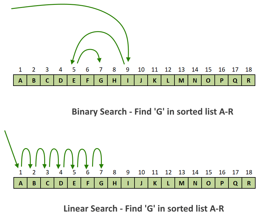
This image provides a great visual summary of the two approaches. Linear search plods along one step at a time, while binary search intelligently jumps through the data.
This graph shows the practical impact of the difference between and complexities.

Relevance to GATE
Understanding algorithmic complexity and the trade-offs between algorithms is crucial for the GATE exam. You won't just be asked to implement them, but to analyze them.
Searching and Sorting Algorithm Notes for GATE Exam
This page from GeeksforGeeks contains some previously asked GATE questions related to searching and sorting. Take a look at questions 4 and 6.
Scroll down to the section titled 'Previously Asked Problems of Searching and Sorting on GATE'. Review Question 4 (about sequential search) and Question 6 (about the complexity of binary search). This shows you how these concepts are tested.
As you can see, the questions test your understanding of the average case complexity and the underlying recurrence relation that defines the algorithm's runtime.
Conclusion
Great work today! You have just learned, implemented, and analyzed two of the most fundamental algorithms in computer science.
Key Takeaways:
- Linear Search is a simple, sequential search with a time complexity of . It's easy to implement and works on unsorted data.
- Binary Search is a highly efficient "divide and conquer" algorithm with a time complexity of , but it critically requires the data to be sorted.
- The difference in performance between and is enormous for large datasets.
- Big-O notation is the standard for expressing how an algorithm's runtime scales with the size of its input.
Preview of the Next Lesson:
The power of binary search is unlocked by having sorted data. But how do we get the data sorted in the first place? In our next lesson, we will begin to answer that question by exploring our first sorting algorithms. You will implement and analyze simple sorting algorithms: bubble sort and insertion sort. This will build directly on today's lesson, showing you the cost you have to pay to enable faster searching.