Mixed Strategies and Expected Payoffs

1. The Rationale for Randomization

In many strategic settings, being predictable is a vulnerability. Consider the simple game of Matching Pennies.

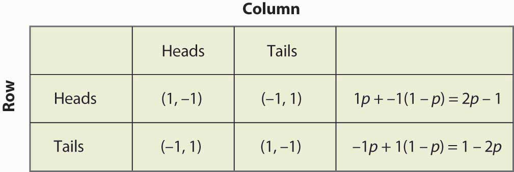
If Player 1 (Row) always chooses Heads, Player 2 (Column) will always choose Tails to win. But if Player 2 always chooses Tails, Player 1 should switch to Tails to win. This cycle of best responses means no pair of pure strategies is stable. The only way to not be exploited is to be unpredictable—to randomize.

To analyze games with random outcomes, we must refine our understanding of payoffs. We move from simple ordinal rankings to a framework of von Neumann-Morgenstern (vNM) preferences. This assumes a player's preferences over lotteries (probabilistic outcomes) can be represented by the expected value of a Bernoulli payoff function over deterministic outcomes. In short, the numbers in our payoff matrices now represent cardinal utilities that can be weighted by probabilities. Given your background in applied mathematics, the theoretical underpinnings of this framework may be of interest.

2. Defining Mixed Strategies

A mixed strategy for a player is a probability distribution over their set of pure strategies. If a player has a set of pure strategies $A_i=\{a_{i1},a_{i2},\dots ,a_{ik}\}$, a mixed strategy ${\sigma }_i$ is a vector of probabilities $({\sigma }_i(a_{i1}),{\sigma }_i(a_{i2}),\dots ,{\sigma }_i(a_{ik}))$ where each ${\sigma }_i(a_{ij})\ge 0$ and ${\sum }_{j=1}^k{\sigma }_i(a_{ij})=1$.

A pure strategy is simply a degenerate mixed strategy where one probability is 1 and all others are 0.

The set of all possible mixed strategies for a player forms a convex set. For a player with $m$ pure strategies, this set can be visualized as a standard simplex in ${\mathbb{R}}^{m-1}$. Given your expertise in informatics and mathematics, the concise representation of mixed strategies and payoffs using linear algebra will be particularly useful.

3. Computing Expected Payoffs

The central task when analyzing mixed strategies is to compute a player's expected payoff. This is the probability-weighted average of the payoffs a player receives across all possible outcomes of the game.

The process involves three steps:

1. For each possible outcome (i.e., each cell in the payoff matrix), calculate its probability of occurring by multiplying the probabilities with which each player chooses the corresponding pure strategy.
2. For a specific player, multiply the probability of each outcome by that player's payoff in that outcome.
3. Sum these values across all outcomes to find the player's total expected payoff.

The following video provides a clear, practical demonstration of this calculation using the Battle of the Sexes game.

Matrix Formulation

This calculation can be expressed more elegantly using matrix notation. Let Player 1's mixed strategy be a row vector $x$ and Player 2's be a column vector $y$. If Player 1's payoff matrix is $A$ and Player 2's is $B$, then their expected payoffs, $U_1$ and $U_2$, are:

$U_1(x,y)=xAy$
$U_2(x,y)=xBy$

This formulation is not just notationally convenient; it is the standard for computational and algorithmic game theory.

Example: Battle of the Sexes

Let's use the game from the video, which is a variant of the Battle of the Sexes.

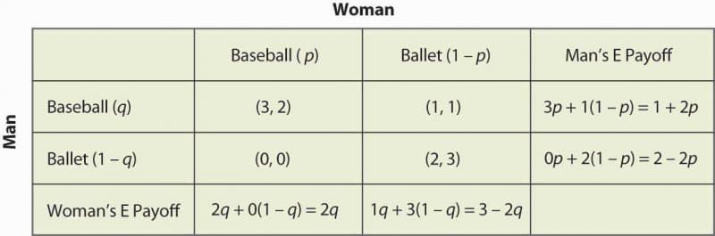
Let's use the mixed strategies identified in the next lesson's material: The Man (Player 1) chooses Baseball with probability $q=2/3$ and Ballet with probability $1-q=1/3$. The Woman (Player 2) chooses Baseball with probability $p=1/3$ and Ballet with probability $1-p=2/3$.

The Man's expected payoff is:

Wait, something is not right in my manual calculation compared to the video. Let's re-verify the video's calculation. The video uses different payoffs and probabilities. Let's stick to the matrix in the image LINK and its notation.

Let's compute the Man's expected payoff if he plays pure Baseball (q=1) against the Woman's mix (p, 1-p):
$E_{Man}(\text{Baseball},p)=3p+1(1-p)=2p+1$
And if he plays pure Ballet (q=0):
$E_{Man}(\text{Ballet},p)=0p+2(1-p)=2-2p$
His total expected payoff for playing the mix $(q,1-q)$ is a weighted average:
$U_{Man}(q,p)=q\cdot E_{Man}(\text{Baseball},p)+(1-q)\cdot E_{Man}(\text{Ballet},p)=q(2p+1)+(1-q)(2-2p)$
This ability to calculate the expected payoff of a pure strategy against an opponent's mixed strategy is fundamental.

4. From Payoffs to Best Responses

The reason we compute expected payoffs is to determine a player's best response. A rational player will choose the strategy that maximizes their expected payoff, given their beliefs about what their opponents will do.

Let's revisit the expected payoffs for the Man's two pure strategies against the Woman's mix $p$:

• $E_{Man}(\text{Baseball},p)=2p+1$
• $E_{Man}(\text{Ballet},p)=2-2p$

His best response depends on the value of $p$:

• If $2p+1>2-2p⟹4p>1⟹p>1/4$, his unique best response is to play pure Baseball.
• If $2p+1<2-2p⟹p<1/4$, his unique best response is to play pure Ballet.
• If $2p+1=2-2p⟹p=1/4$, he is indifferent between Baseball and Ballet. In this specific case, any mixed strategy, including pure Baseball, pure Ballet, or any mix between them, is a best response.

This observation is the key to finding mixed strategy equilibria, which is the topic of our next lesson. An essential property of expected payoffs in two-action games is their linearity, which leads directly to this "all-or-nothing" or "indifference" structure for best responses.

Conclusion

This lesson has laid the groundwork for analyzing games of uncertainty. We have moved beyond the deterministic world of pure strategies and equipped ourselves with the necessary conceptual and computational tools to handle randomization.

Key Takeaways:

• Mixed strategies are probability distributions over pure strategies, used to model unpredictability and analyze games without pure strategy equilibria.
• Analyzing mixed strategies requires vNM preferences, where payoffs are cardinal utilities whose expected values represent preferences over lotteries.
• The expected payoff of a mixed strategy profile is the probability-weighted average of the payoffs of all possible outcomes.
• This calculation can be performed algorithmically or expressed compactly using matrix notation ($xAy$).
• A player's best response is the strategy that maximizes their expected payoff. For any given opponent strategy, a player's best response will be a pure strategy unless they are indifferent between multiple pure strategies.

In our next lesson, we will leverage this final point—the principle of indifference—to develop a powerful method for computing the mixed strategy Nash Equilibrium in 2x2 games.