Welcome to your seventh and final lesson in the Graph Algorithms module.
In our last few lessons, we focused on finding the shortest path from a single source, culminating with the Bellman-Ford algorithm, which robustly handles negative edge weights. Today, we shift our focus from finding the shortest path between two points to solving a different, equally fundamental problem: finding the most efficient way to connect all points in a network.
This lesson introduces the concept of a Minimum Spanning Tree (MST). You will learn to implement the two classic greedy algorithms used to find it: Kruskal's and Prim's. Mastering these is essential for network design problems and showcases a powerful application of the greedy algorithmic paradigm.
The Five Concepts for Today
- The Minimum Spanning Tree Problem: Defining what an MST is and where it's used.
- Kruskal's Algorithm: The edge-centric approach, using a Disjoint Set Union (DSU) data structure for cycle detection.
- Prim's Algorithm: The vertex-centric approach, growing the MST outward from a single source, much like Dijkstra's algorithm.
- Python Implementation & Complexity: Implementing both algorithms and analyzing their performance.
- Interview Deep Dive: Comparing Kruskal's vs. Prim's and understanding the trade-offs for sparse vs. dense graphs.
Concept 1: What is a Minimum Spanning Tree?
Technical Explanation
Given a connected, undirected, weighted graph, a spanning tree is a subgraph that connects all the vertices together with the minimum possible number of edges () and contains no cycles. A graph can have many different spanning trees.
A Minimum Spanning Tree (MST) is the specific spanning tree that has the minimum possible sum of edge weights.
An MST must satisfy three properties:
- Connects all vertices: Every node in the graph is reachable from every other node within the MST.
- Acyclic: It contains no cycles. A graph with vertices and edges that is connected is guaranteed to be a tree (and thus acyclic).
- Minimum total weight: The sum of the weights of all edges in the tree is less than or equal to the total weight of any other spanning tree.
Algorithms Toolkit: A Python Developer's Guide to 16 Core ...
The following article provides a crisp definition of a Minimum Spanning Tree and a great real-world analogy to frame the problem.
Read the subsection '10. Minimum Spanning Tree (MST): Building the Most Efficient Network,' specifically the part under 'What It Is.'
Metaphor: The Neighborhood Cable Company
Imagine you're a company tasked with laying fiber optic cable to connect a new neighborhood of houses. The houses are the vertices, and the possible paths between houses are the edges, weighted by the cost to dig and lay cable along that path.
Your goal is to connect every single house to the network (spanning). You want to do this using the least amount of cable possible to minimize cost (minimum weight). You also don't want to create any redundant loops, as that's just wasted cable (acyclic). The final layout of your cables would be a Minimum Spanning Tree.
Concept 2: Kruskal's Algorithm - The Edge-Centric Approach
Technical Explanation
Kruskal's algorithm takes an edge-centric greedy approach. It doesn't grow the tree from one point; instead, it builds a "forest" of trees that gradually merge into a single MST.
The algorithm is beautifully simple:
- Create a list of all edges in the graph.
- Sort the list of edges in non-decreasing order of their weights.
- Initialize an empty MST.
- Iterate through the sorted edges. For each edge :
- If adding the edge does not form a cycle with the edges already in the MST, add it.
- Otherwise, discard the edge.
- Stop when the MST has edges.
The critical challenge is: How do we efficiently check if adding an edge forms a cycle? This is where the Disjoint Set Union (DSU) data structure comes in. A DSU (or Union-Find) tracks a set of elements partitioned into a number of disjoint (non-overlapping) subsets. In our case, each subset is a connected component of vertices.
find(v): Determines which subset (or component) a vertexvbelongs to.union(u, v): Merges the subsets containinguandv.
Before adding an edge , we check if find(u) equals find(v). If they are already in the same component, adding the edge would form a cycle. If not, we add the edge and call union(u, v) to merge their components.
Kruskal's Algorithm Visually Explained | Disjoint Sets | Union By Rank | Path Compression
This video provides an excellent visual explanation of Kruskal's algorithm and introduces the role of the Disjoint Set data structure for cycle detection.
Watch from the beginning to 01:57. Focus on how the algorithm sorts edges and uses the concept of 'sets' to decide whether to include an edge or not.
For peak performance, the DSU is implemented with two key optimizations: path compression and union by rank/size. Path compression flattens the tree structure during find operations, while union by rank/size ensures the trees remain balanced during union operations. Together, they make DSU operations almost constant time on average.
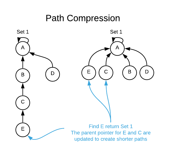
For a deeper, optional dive into DSU, the cp-algorithms article (ID=[LINK](https://cp-algorithms.com/data_structures/disjoint_set_union.html)) is a fantastic resource, particularly the sections on path compression and union by rank.
Concept 3: Prim's Algorithm - The Vertex-Centric Approach
Technical Explanation
Prim's algorithm takes a vertex-centric greedy approach, which should feel familiar after studying Dijkstra's. It grows a single MST from an arbitrary starting vertex.
The algorithm works as follows:
- Initialize an empty MST.
- Choose an arbitrary starting vertex
s. - Maintain a priority queue of edges that connect vertices inside the growing MST to vertices outside of it. The priority is the edge weight (lowest first).
- While the MST doesn't include all vertices:
- Extract the minimum-weight edge from the priority queue, where
uis in the MST andvis not. - Add vertex
vand edge to the MST. - For all edges connected to
v, if they lead to a vertex not yet in the MST, add them to the priority queue.
- Extract the minimum-weight edge from the priority queue, where
The greedy choice here is always picking the cheapest "bridge" edge from the current connected component to an unconnected vertex. Because of its structural similarity to Dijkstra's, a priority queue is the natural data structure to implement it efficiently.
Prim's Algorithm Visually Explained | Minimum Spanning Tree
This video visually demonstrates Prim's algorithm, highlighting the use of a priority queue to select the next cheapest edge from the 'fringe' of the growing tree.
Watch from the beginning to 01:48. Pay attention to how the algorithm expands from a single node and how the set of 'candidate' edges changes at each step.

Concept 4: Python Implementations & Complexity Analysis
Kruskal's Algorithm Implementation
Kruskal's requires a DSU helper class. Here is a full implementation.
# Helper class for Disjoint Set Union (DSU)
class DSU:
    def __init__(self, vertices):
        self.parent = {v: v for v in vertices}
        self.rank = {v: 0 for v in vertices}

    def find(self, v):
        if self.parent[v] != v:
            # Path compression
            self.parent[v] = self.find(self.parent[v])
        return self.parent[v]

    def union(self, u, v):
        root_u = self.find(u)
        root_v = self.find(v)
        if root_u != root_v:
            # Union by rank
            if self.rank[root_u] > self.rank[root_v]:
                self.parent[root_v] = root_u
            elif self.rank[root_u] < self.rank[root_v]:
                self.parent[root_u] = root_v
            else:
                self.parent[root_v] = root_u
                self.rank[root_u] += 1
            return True
        return False

def kruskals_algorithm(graph_edges, vertices):
    """
    Finds the MST of a graph using Kruskal's algorithm.
    Args:
        graph_edges: A list of edges [u, v, weight].
        vertices: A list of all vertices in the graph.
    Returns:
        A list of edges in the MST and its total cost.
    """
    # 1. Sort all edges by weight
    graph_edges.sort(key=lambda item: item[2])

    dsu = DSU(vertices)
    mst = []
    mst_cost = 0

    # 2. Iterate through sorted edges
    for u, v, weight in graph_edges:
        # 3. If adding the edge doesn't form a cycle, add it
        if dsu.union(u, v):
            mst.append((u, v, weight))
            mst_cost += weight
            # Optimization: stop when MST is complete
            if len(mst) == len(vertices) - 1:
                break

    return mst, mst_cost

# --- Example Usage ---
vertices = ['A', 'B', 'C', 'D', 'E', 'F']
edges = [['A', 'B', 2], ['A', 'F', 3], ['B', 'C', 5],
         ['B', 'D', 2], ['C', 'D', 1], ['D', 'E', 4],
         ['D', 'F', 6], ['E', 'F', 5]]

mst_kruskal, cost_kruskal = kruskals_algorithm(edges, vertices)
print(f"Kruskal's MST: {mst_kruskal}, Total Cost: {cost_kruskal}")
# Expected: Edges with weights 1, 2, 2, 3, 4. Total Cost: 12
- Time Complexity: . The dominant operation is sorting the edges. The DSU operations, with optimizations, have an amortized complexity that is nearly constant (, where is the inverse Ackermann function), so they don't impact the overall complexity.
- Space Complexity: . We need space for the edge list and the DSU parent/rank arrays.
Prim's Algorithm Implementation
Prim's requires a priority queue, which is easily implemented with Python's heapq module.
import heapq

def prims_algorithm(graph, start_vertex):
    """
    Finds the MST of a graph using Prim's algorithm.
    Args:
        graph: An adjacency list representation {vertex: [(neighbor, weight), ...]}.
        start_vertex: The vertex to start from.
    Returns:
        A list of edges in the MST and its total cost.
    """
    mst = []
    mst_cost = 0
    visited = set([start_vertex])

    # Priority queue stores (weight, u, v)
    edges_pq = []
    for neighbor, weight in graph[start_vertex]:
        heapq.heappush(edges_pq, (weight, start_vertex, neighbor))

    # Loop until we have V-1 edges in the MST
    while edges_pq and len(mst) < len(graph) - 1:
        weight, u, v = heapq.heappop(edges_pq)

        if v not in visited:
            visited.add(v)
            mst.append((u, v, weight))
            mst_cost += weight

            # Add new edges from the newly added vertex v
            for next_neighbor, next_weight in graph[v]:
                if next_neighbor not in visited:
                    heapq.heappush(edges_pq, (next_weight, v, next_neighbor))

    return mst, mst_cost

# --- Example Usage ---
adj_list = {
    'A': [('B', 2), ('F', 3)],
    'B': [('A', 2), ('C', 5), ('D', 2)],
    'C': [('B', 5), ('D', 1)],
    'D': [('B', 2), ('C', 1), ('E', 4), ('F', 6)],
    'E': [('D', 4), ('F', 5)],
    'F': [('A', 3), ('D', 6), ('E', 5)]
}

mst_prim, cost_prim = prims_algorithm(adj_list, 'A')
print(f"Prim's MST: {mst_prim}, Total Cost: {cost_prim}")
# Expected: Edges with weights 2, 2, 1, 3, 4. Total Cost: 12
- Time Complexity: . In the worst case, every edge is added to the priority queue. Heap operations (push and pop) take . The size of the priority queue can go up to , but a tighter bound is because an edge is added once for each vertex it connects to, and heap operations are since at most vertices are considered.
- Space Complexity: . For the adjacency list, visited set, and the priority queue.
Concept 5: Interview Deep Dive - Kruskal's vs. Prim's
In an interview, you'll be expected to justify your choice of algorithm. The decision between Kruskal's and Prim's hinges on graph density and representation.
| Aspect | Kruskal's Algorithm | Prim's Algorithm |
|---|---|---|
| Greedy Choice | Add the next cheapest edge that doesn't form a cycle. | Add the cheapest edge connecting the MST to an unvisited vertex. |
| Structure | Builds a "forest" of components that merge into one tree. | Grows a single tree from a starting vertex. |
| Data Structure | Disjoint Set Union (DSU) | Priority Queue |
| Time Complexity | ||
| Best For | Sparse graphs ( is close to ). Also useful if the graph is disconnected (finds an MST for each component). | Dense graphs ( is close to ). |
Why the sparse vs. dense distinction?
- For a sparse graph, is roughly proportional to . Kruskal's becomes , making it comparable to or faster than Prim's.
- For a dense graph, approaches . Kruskal's complexity becomes . Prim's remains . While asymptotically similar, Prim's is often faster in practice on dense graphs because it avoids the overhead of sorting all edges upfront and uses a priority queue that never holds more than "best" edges at once in some implementations. The standard interview answer is: Kruskal's for sparse, Prim's for dense.
Test your understanding!
You are hired by a social media company. They want to run a "friend-of-a-friend" analysis to find the most efficient way to connect a small, targeted group of influential users. The graph of all users is enormous, but you are given only the list of connections between the target users. This results in a graph that is potentially disconnected and sparse. Which MST algorithm would be more suitable and why?
Show answer
Kruskal's algorithm is more suitable.
- Disconnected Graph: The problem statement implies the graph of target users might be disconnected. Kruskal's naturally handles this by producing a "minimum spanning forest"—one MST for each connected component of users. Prim's would only find an MST for the component containing its start vertex.
- Graph Representation: You are given an edge list ("list of connections"), which is the exact input Kruskal's is designed for. Prim's works more naturally with an adjacency list, which you would have to build first.
- Sparsity: The graph is likely sparse, where Kruskal's is most efficient.
Conclusion
Today, you've mastered two fundamental greedy algorithms for finding Minimum Spanning Trees. You've seen how a problem can be solved from two different perspectives: edge-centric (Kruskal's) and vertex-centric (Prim's), and you've learned about the powerful DSU data structure that enables Kruskal's algorithm.
Key Takeaways:
- An MST is the cheapest way to connect all vertices in a weighted, undirected graph.
- Kruskal's algorithm sorts all edges and adds them greedily, using a DSU to prevent cycles. It excels on sparse graphs.
- Prim's algorithm grows a tree from a start node, using a priority queue to always add the cheapest connecting edge. It is preferred for dense graphs.
- The choice between them depends on graph density, its representation (edge list vs. adjacency list), and whether it might be disconnected.
Preview of the Next Module:
This lesson was the perfect bridge to our next module: Dynamic Programming and Greedy Algorithms. Kruskal's and Prim's are canonical examples of greedy algorithms. In our next lesson, we will formalize what makes a problem suitable for a greedy approach by exploring the concepts of "optimal substructure" and the "greedy-choice property," which you've just seen in action.