Welcome to your third lesson in the System Design: Scalability, Caching, and Storage module. In our previous lessons, we learned to estimate a system's capacity needs and then designed its "front door"—the API. We now have a contract for how clients will talk to our system and an idea of the load to expect. The next logical question is: how do we build an infrastructure that can actually handle that load, especially as it grows?
Today, we'll tackle one of the most fundamental concepts in system design: scalability. You will learn to analyze the two primary strategies for growing a system—horizontal scaling and vertical scaling—and understand their deep architectural trade-offs. This knowledge is non-negotiable for designing systems that can serve millions of users, a core competency tested in elite engineering interviews.
1. The Two Paths to Growth: Vertical vs. Horizontal Scaling
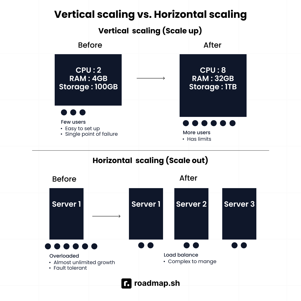
When a single server can no longer handle the incoming request volume, you have two choices: make the server more powerful, or get more servers. This is the fundamental dilemma of scaling.
- Vertical Scaling (Scaling Up): This strategy involves increasing the resources of a single server. You add more CPU cores, more RAM, or faster storage (like moving from HDD to NVMe SSDs) to the existing machine.
- Horizontal Scaling (Scaling Out): This strategy involves adding more servers to your pool of resources. Instead of one powerful machine, you distribute the load across multiple, often less powerful, commodity machines.
To get a quick and clear overview of these concepts, let's start with a short video.
Vertical Vs Horizontal Scaling: Key Differences You Should Know
The ByteByteGo channel provides a concise, animated explanation of vertical and horizontal scaling, including their primary advantages and disadvantages. This will give us a solid foundation.
Watch the segment from 00:13 to 02:24. As you watch, focus on the core definitions and the initial list of pros and cons for each approach.
The Metaphor: The Programmer and the Project
- Vertical Scaling is like upgrading your single laptop. Your project is running slow, so you replace your 4-core i5 processor with a 16-core i9, upgrade from 16GB to 64GB of RAM, and get a faster SSD. You're still one person working on one machine, but that machine is now a beast. It's simple, and all your files are in one place.
- Horizontal Scaling is like hiring two new programmers and giving them identical laptops. Now, three people can work on different parts of the project simultaneously. You need a project manager (a load balancer) to distribute tasks and a way for everyone to share their work (a distributed filesystem or database), but you can get much more done in parallel.
2. The Architectural Trade-Offs
Choosing between scaling up and scaling out involves a complex set of trade-offs that impact reliability, cost, and maintainability. A senior engineer must be able to articulate these clearly.
To deepen our understanding of these trade-offs, let's watch another video that breaks them down across several key dimensions.
System Design BASICS: Horizontal vs. Vertical Scaling
This video from Gaurav Sen provides a more in-depth comparison, touching on factors like data consistency, network communication, and resilience, which are critical in real-world distributed systems.
Watch the section from 04:03 to 06:21. Pay close attention to his five points of comparison: load balancing, resilience, inter-server communication, data consistency, and hardware limits.
Let's synthesize this information into a detailed table, which is a common way to present trade-offs in a system design interview.
| Dimension | Vertical Scaling (Scale Up) | Horizontal Scaling (Scale Out) | Architectural Implication & "So What?" |
|---|---|---|---|
| Fault Tolerance | Low. Creates a Single Point of Failure (SPOF). If the machine fails, the entire system is down. | High. The system is resilient. If one server fails, the load balancer redirects traffic to healthy servers. | Horizontal scaling is essential for high-availability systems (e.g., e-commerce checkout, messaging apps) where downtime is unacceptable. Vertical scaling is a major risk for any critical service. |
| Implementation Complexity | Simple. Managing one machine is straightforward. No need for load balancers or complex networking. | Complex. Requires a load balancer, service discovery, and mechanisms for data replication/synchronization. | The operational overhead of horizontal scaling is significant. You move from managing a machine to managing a distributed system, which requires specialized expertise and tooling (like Kubernetes). |
| Data Consistency | High (Strong Consistency). All operations occur on a single machine, often within a single process. | Challenging. Maintaining consistency across multiple machines requires complex protocols and often leads to eventual consistency. | This is a crucial point for databases. A vertically scaled database (like a traditional SQL server) is easier to keep consistent. A horizontally scaled (sharded) database introduces challenges in maintaining transactional integrity across nodes. |
| Performance & Limits | Limited by the maximum power of a single machine. Diminishing returns on cost at the high end. | Virtually unlimited. You can theoretically add an infinite number of servers. Performance can be degraded by network latency. | Vertical scaling eventually hits a hard physical and financial ceiling. Horizontal scaling is the only viable path for "web-scale" systems like Google Search or Netflix streaming, which handle traffic far beyond the capacity of any single machine. |
| Cost Model | High upfront cost (CAPEX). High-end servers are exponentially more expensive. | Pay-as-you-go (OPEX). Commodity hardware is cheap, and cloud providers make it easy to add/remove instances. | Horizontal scaling aligns better with the cloud computing model. You can dynamically scale your capacity to match demand (auto-scaling), which is more cost-effective than maintaining an oversized server that is idle most of the time. |
Real-World Examples:
- Vertical Scaling: High-frequency trading systems or large, monolithic databases in traditional finance often run on extremely powerful, vertically scaled mainframes to ensure the highest single-thread performance and strong consistency.
- Horizontal Scaling: Almost every large-scale web service you use—Google, Meta, Netflix, Amazon—is built on the principle of horizontal scaling, distributing work across tens of thousands of commodity servers.
3. The Theoretical Limit: Why You Can't Just Add More Servers
It seems like horizontal scaling is the clear winner for large systems. But is it as simple as "add more servers, get more performance"? The answer is no. A fundamental law of computing explains why.
Amdahl's Law
Proposed by computer architect Gene Amdahl in 1967, Amdahl's Law provides a formula for the theoretical maximum speedup you can achieve by parallelizing a task. Its core insight is that every program has a serial component that cannot be parallelized, and this serial part becomes the ultimate bottleneck.
The formula for speedup () is:
Where:
- is the number of processors (or servers).
- is the fraction of the program that is serial (cannot be parallelized).
- is the fraction that can be parallelized.
The Metaphor: The Pizza Kitchen
Imagine you have a pizza recipe that takes 40 minutes for the dough to rise (serial part) and 5 minutes to add toppings (parallelizable part).
- One Chef: Total time = 40 + 5 = 45 minutes.
- Five Chefs: You can have 5 chefs add toppings simultaneously. This takes 5 chefs * (5 mins / 5) = 1 minute. But the dough still needs 40 minutes to rise. Total time = 40 + 1 = 41 minutes.
- Infinite Chefs: Even with infinite chefs, the topping time approaches zero, but the 40-minute rising time remains. The total time can never be less than 40 minutes.
The dough rising time is the serial fraction (), and it dictates your maximum speedup.
To dig deeper into this and other formal metrics, the "Parallel Scaling Guide" is an excellent, mathematically rigorous resource.
This guide from the Colorado School of Mines, while written for high-performance computing, provides a perfect 'under the hood' explanation of the theory behind scaling. We'll focus on Amdahl's Law.
Read the section titled 'Basic Theory', focusing specifically on the subsection 'Amdahl’s Law'. Understand the formula and the implication of the serial fraction (Fs).
Test your understanding! (Interview-Style Question)
You are leading a team that has just scaled your web application's server fleet from 10 to 100 instances (a 10x increase). However, performance testing shows that the system's throughput only improved by 3x. Your manager is concerned. What is the most likely theoretical reason for these diminishing returns, and what does it imply about your application's architecture?
Show answer
The most likely reason is Amdahl's Law. My explanation would be:
"The observed 3x speedup on a 10x resource increase strongly suggests that our application has a significant serial component in its workload. According to Amdahl's Law, the maximum speedup is limited by the portion of the work that cannot be parallelized.
Let's do a quick calculation. If when we scale from 10 to 100 machines (a 10x increase in the parallel part, so ), we can estimate the serial fraction :
Solving for , we get approximately , or 26%.
This implies that about a quarter of our request processing time is spent on a task that cannot be distributed across our servers. This bottleneck could be:
- A database transaction on a single, non-sharded database.
- A call to a slow, third-party legacy service.
- Contention for a shared lock or resource.
My next step would be to use profiling and tracing tools (like Jaeger or Zipkin) to identify and quantify this serial bottleneck. The goal would be to reduce this fraction, which would unlock better scalability as we add more machines."
4. Strong vs. Weak Scaling: What Are You Trying to Achieve?
The term "scaling" can mean two different things, and the distinction is crucial for designing data platforms.
- Strong Scaling: Aims to solve the same size problem faster by adding more resources. The goal is to reduce latency.
- Example: A web request takes 500ms. By adding more servers to parallelize the backend work, you aim to reduce the response time to 100ms. The problem (one request) stays the same size.
- Weak Scaling: Aims to solve a proportionally larger problem in the same amount of time by adding more resources. The goal is to increase throughput.
- Example: A MapReduce job processes 1TB of data in 1 hour on 100 nodes. With weak scaling, you should be able to process 10TB of data in 1 hour on 1000 nodes. The problem size grows with the resources.
This distinction is formally defined in the same "Parallel Scaling Guide." It's worth reading the definitions for "Strong Scaling" and "Weak Scaling" in resource LINK (sections 3 and 4) to solidify your understanding.
For the AI/ML and data platforms you're interested in, weak scaling is often the more important metric. You want to know that your architecture can handle growing datasets by simply adding more nodes.
5. The Real World: Contention, Coherency, and the Hybrid Model
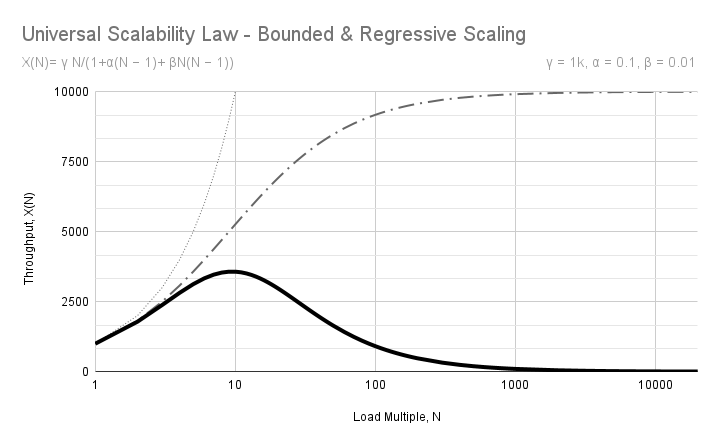
Amdahl's Law is a bit simplistic. It assumes the serial fraction is constant. In reality, as you add more servers, the work required to coordinate them often increases. This leads to two new sources of overhead:
- Contention (): Waiting for a shared resource that cannot be used concurrently, like a lock on a database row.
- Coherency (): The overhead of making sure all servers have a consistent view of the data. This involves things like cache invalidation messages or data replication traffic.
The Universal Scalability Law (USL) models this reality.
The Hybrid Approach: Diagonal Scaling
Given the trade-offs, modern systems rarely choose one strategy exclusively. The most common and effective approach is a hybrid one, sometimes called diagonal scaling:
- Start with Vertical Scaling: Use the most powerful single machine that is cost-effective. This simplifies your architecture initially.
- Then, Scale Horizontally: Once a single powerful machine is not enough, or becomes prohibitively expensive, begin scaling out horizontally using these powerful machines as your building blocks.
This gives you the best of both worlds: strong performance on each individual node and the near-infinite scalability of a distributed architecture.
Python Code: Simulating Amdahl's Law
While we can't build a full distributed system here, we can use Python to visualize the impact of Amdahl's Law and understand why your 10x resource investment might not yield a 10x return.
import matplotlib.pyplot as plt
import numpy as np

def amdahls_law_speedup(P, Fs):
    """
    Calculates the theoretical speedup based on Amdahl's Law.

    Args:
        P (np.array): An array of processor counts.
        Fs (float): The serial fraction of the code (0 to 1).

    Returns:
        np.array: The calculated speedup for each processor count.
    """
    return 1 / (Fs + (1 - Fs) / P)

# Set up processor counts from 1 to 1024
processors = np.array([2**i for i in range(11)]) # 1, 2, 4, ..., 1024

# Serial fractions to test
serial_fractions = [0.001, 0.01, 0.05, 0.1, 0.25]

plt.figure(figsize=(12, 8))

# Plot ideal linear speedup
plt.plot(processors, processors, 'k--', label='Ideal Linear Speedup')

# Plot Amdahl's Law for different serial fractions
for fs in serial_fractions:
    speedup = amdahls_law_speedup(processors, fs)
    plt.plot(processors, speedup, marker='o', linestyle='-', label=f'Fs = {fs*100}%')

plt.title("Amdahl's Law: The Limit of Parallel Speedup", fontsize=16)
plt.xlabel("Number of Processors (P)", fontsize=12)
plt.ylabel("Speedup", fontsize=12)
plt.xscale('log', base=2)
plt.yscale('log', base=2)
plt.xticks(processors, labels=[str(p) for p in processors])
plt.grid(True, which="both", ls="--")
plt.legend()
plt.show()
Running this code will generate a plot showing that as the serial fraction (Fs) increases, the speedup curve flattens dramatically, visually demonstrating the bottleneck.
Conclusion
You now have a multi-layered understanding of scalability. You've gone from the basic definitions to the deep theoretical laws that govern real-world systems.
Key Takeaways:
- Vertical Scaling (Up): More power, one machine. Simple, consistent, but limited and creates a single point of failure.
- Horizontal Scaling (Out): More machines. Resilient, virtually limitless, but complex to manage.
- Amdahl's Law: Your system's scalability is ultimately capped by its serial fraction. You cannot achieve perfect linear speedup.
- Strong vs. Weak Scaling: Are you trying to reduce latency (strong) or increase throughput for larger problems (weak)? The answer dictates your design and testing strategy.
- Hybrid Model: The most practical approach is diagonal scaling: use powerful nodes and add more of them as needed.
Next Lesson Preview
We've established that scaling out with more servers is the path to building large systems. But this strategy only works if we make each server's work as efficient as possible. One of the most powerful tools for this is caching. By storing frequently accessed data in a fast, in-memory layer, we can dramatically reduce the load on our databases and backend services.
In the next lesson, we will get hands-on and implement a Least Recently Used (LRU) Cache from scratch using a hash map and a doubly linked list. This is a classic and frequent problem in top-tier coding interviews.