Analyzing Algorithm Efficiency with Big O, Omega, and Theta Notations

Concept 1: What is Algorithm Analysis?

At its core, algorithm analysis isn't about measuring how fast a program runs on your specific laptop. That time can change based on your computer's speed, the programming language, or even other programs running in the background. Instead, we need a universal way to talk about an algorithm's efficiency that is independent of hardware.

Technical Explanation

Algorithm analysis focuses on understanding how an algorithm's resource requirements—primarily time (CPU operations) and space (memory)—grow as the size of the input grows. We call the input size n. This is known as Asymptotic Analysis. We're not interested in the exact number of seconds an algorithm takes, but rather in its rate of growth. An algorithm that is fast for small n might become unusably slow for large n, and this is precisely what we need to predict and avoid when building scalable systems.

Metaphor: The Bookshelf

Imagine you have a bookshelf with n books.

• Task 1: Checking if the bookshelf is empty. This takes a single glance, regardless of whether there are 0, 10, or 1,000 books. The effort is constant.
• Task 2: Reading the title of every book. If you double the number of books, this task will take you about twice as long. The effort grows linearly with the number of books.
• Task 3: Checking for a duplicate book. You might have to take the first book and compare it to all others, then the second book and compare it to all others, and so on. If you double the number of books, this task will take much more than twice as long. The effort grows quadratically.

Asymptotic analysis gives us the language to describe these different growth rates.

Industry Application

When Google indexes the web, n (the number of web pages) is in the trillions. If their indexing algorithm's runtime grew quadratically with n, it would be computationally impossible to run. They must use algorithms whose runtime scales gracefully (e.g., linearly or near-linearly) with the massive amount of data they process.

Interview Question

"Why do we use asymptotic notations like Big O instead of just timing our code with a stopwatch?"

Answer: Stopwatch timing is unreliable because it depends on the specific hardware, the current load on the system, the programming language, and the compiler. Asymptotic analysis provides a hardware-agnostic, mathematical way to describe the fundamental scalability of an algorithm, which is what truly matters for predicting its performance on very large inputs.

Concept 2: Big O Notation ($O$) — The Upper Bound

Big O is the most common and important notation you will encounter. It describes the worst-case scenario or provides an upper bound on an algorithm's time complexity.

Technical Explanation

When we say an algorithm is $O(g(n))$, we are making a guarantee: for a sufficiently large input n, the algorithm's runtime will not grow faster than a constant multiple of $g(n)$.

The formal definition is key to understanding this "under the hood":
A function $f(n)$ (representing your algorithm's exact step count) is in $O(g(n))$ if there exist positive constants $c$ and $n_0$ such that for all $n\ge n_0$, the following inequality holds:
$0\le f(n)\le c\cdot g(n)$

• $g(n)$ is the function we are bounding against (e.g., $n$, $n^2$).
• $c$ is a constant factor. The definition allows us to pick a $c$ large enough to make the inequality true. This is why we drop constants in Big O notation (e.g., $O(2n)$ simplifies to $O(n)$).
• $n_0$ is the input size after which the upper bound always holds. This is why we drop lower-order terms. For large $n$, the highest-order term dominates the growth rate (e.g., in $n^2+100n$, the $n^2$ term eventually grows much faster than $100n$).

To get a strong visual and intuitive grasp of this definition, the following video is excellent.

Metaphor: Planning a Road Trip

Big O is like telling a friend you'll arrive at your destination in at most 5 hours. You might hit no traffic and arrive in 4 hours, but you're providing a guaranteed upper limit on the travel time. The actual time will be less than or equal to 5 hours.

Python Code: Analyzing a Simple Loop

Let's analyze a function that finds an element in a list (linear search).

def linear_search(data_list, target):
    """
    Returns True if target is in the list, False otherwise.
    n = len(data_list)
    """
    for item in data_list:  # This loop runs at most n times
        if item == target:
            return True
    return False

# Example usage:
my_list = [1, 5, 8, 10, 23, 42]
# In the worst case, we search for 42 or a number not in the list.
# The loop will run len(my_list) = 6 times.

In the worst-case scenario (the target is the last element or not in the list), the for loop will run n times, where n is the number of items in data_list. Therefore, the time complexity is $O(n)$.

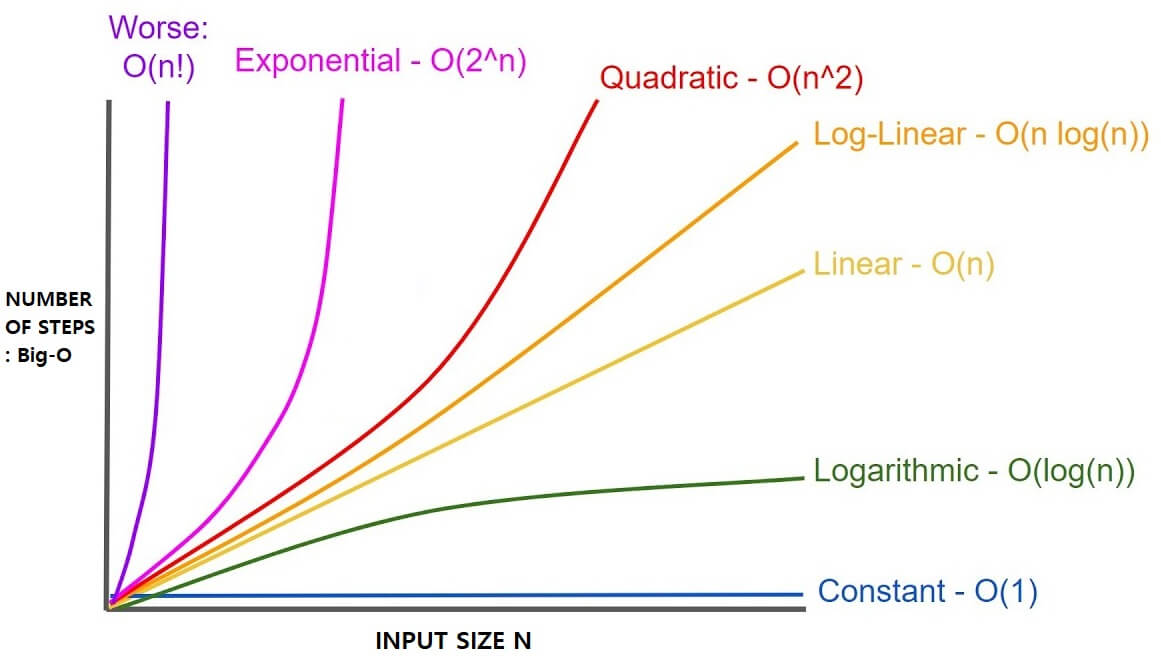
Concept 3: Common Complexity Classes

Algorithms are categorized into "complexity classes" based on their Big O notation. Knowing these is like knowing the vocabulary of performance.

Technical Explanation

Here are the most common classes, from fastest to slowest growing:

• $O(1)$ — Constant Time: The runtime does not change with the input size.
  • Example: Accessing an element in an array by its index (my_array[5]).
• $O(\log n)$ — Logarithmic Time: The runtime grows very slowly. Every time you double the input size, the work only increases by one unit.
  • Example: Binary search on a sorted array.
• $O(n)$ — Linear Time: The runtime grows proportionally to the input size.
  • Example: Iterating through all elements in a list.
• $O(n\log n)$ — Log-Linear Time: Slightly worse than linear. Most efficient sorting algorithms fall into this category.
  • Example: Merge Sort, Quick Sort.
• $O(n^2)$ — Quadratic Time: The runtime grows by the square of the input size. Often involves nested loops over the same data.
  • Example: A simple algorithm to find pairs of elements in a list.
• $O(2^n)$ — Exponential Time: The runtime doubles with each new element added to the input. Quickly becomes unusable for even small n.
  • Example: Finding all subsets of a set.

Industry Application

A naive "People You May Know" feature on a social network might compare every user to every other user, an $O(n^2)$ operation. For a platform with millions of users ($n$), this is impossible. Real systems use much more sophisticated graph algorithms and indexing to make this recommendation task feasible, often approximating it with near-linear time complexity.

Concept 4: Big Omega ($\Omega$) and Big Theta ($\Theta$)

While Big O gives the upper bound (worst case), Big Omega and Big Theta give us a more complete picture by describing the lower bound and tight bound.

Technical Explanation

• Big Omega ($\Omega$): The Lower Bound

  • This describes the best-case scenario. An algorithm is guaranteed to take at least this amount of time.
  • Formal Definition: $f(n)\in \Omega (g(n))$ if there exist positive constants $c$ and $n_0$ such that for all $n\ge n_0$:
    $0\le c\cdot g(n)\le f(n)$

• Big Theta ($\Theta$): The Tight Bound

  • This is the most precise description. It means the algorithm's runtime is bounded both from above and below by the same growth function. This happens when the best-case and worst-case complexities are the same.
  • Formal Definition: $f(n)\in \Theta (g(n))$ if and only if $f(n)\in O(g(n))$ and $f(n)\in \Omega (g(n))$.

Metaphor: Road Trip Revisited

• Big Omega ($\Omega$): "I will arrive in at least 4 hours." (You won't be any faster due to speed limits and distance).
• Big Theta ($\Theta$): "This trip takes about 4.5 hours." (It's tightly bound; it won't be 1 hour, and it won't be 10 hours).

Python Code: Best vs. Worst Case

Let's revisit our linear_search function.

• Best Case: The target is the very first element. The loop runs once. The complexity is $\Omega (1)$.
• Worst Case: The target is the last element or not present. The loop runs n times. The complexity is $O(n)$.

Since the best case ($\Omega (1)$) and worst case ($O(n)$) are different, we cannot describe this algorithm with a single $\Theta$ notation.

Now consider an algorithm to find the maximum value in a list:

def find_max(data_list):
    """
    Returns the maximum value in a non-empty list.
    n = len(data_list)
    """
    if not data_list:
        return None
    
    max_val = data_list[0] # 1 operation
    for i in range(1, len(data_list)): # Loop always runs n-1 times
        if data_list[i] > max_val:
            max_val = data_list[i]
    return max_val

This algorithm must check every element to be sure it has found the maximum. The loop always runs n-1 times. Therefore, its best case and worst case are the same. We can say its complexity is $\Theta (n)$.

Interview Question

"What is the difference between Big O and Big Theta? When would you use one versus the other?"

Answer: "Big O describes the upper bound or worst-case complexity, giving a guarantee that the algorithm won't be slower. Big Theta describes a tight bound, used when the best-case and worst-case complexities are the same. In an interview, I would default to using Big O because it describes the worst-case behavior, which is what we usually care about for scalability. If I determine that the best and worst cases are the same, I might explicitly state that the algorithm is Theta of n, $\Theta (n)$, to be more precise."

Concept 5: Practical Application — Analyzing Iterative Code

Let's put it all together with a clear process for analyzing your own code.

Technical Explanation

To find the Big O complexity of a piece of code, follow these rules:

1. Consecutive Statements: Add the complexities. The largest one dominates.
   • O(n) + O(1) simplifies to O(n).
2. Loops: Multiply the complexity of the loop's body by the number of times the loop runs.
   • A for loop that runs n times with an O(1) body is n * O(1) = O(n).
3. Nested Loops: Multiply the complexities of the inner and outer loops.
   • An outer loop running n times and an inner loop running n times results in O(n * n) = O(n^2).

The final step is always to drop constants and lower-order terms.

Python Code: A Nested Loop Example

Let's analyze a function that finds duplicate items in a list.

def find_duplicates(items):
    # Let n = len(items)
    for i in range(len(items)):         # Rule 3: This outer loop runs n times.
        for j in range(i + 1, len(items)): # Rule 3: This inner loop runs...
                                           # When i=0, it runs n-1 times.
                                           # When i=1, it runs n-2 times.
                                           # ...
                                           # On average, it runs about n/2 times.
            if items[i] == items[j]:
                print("Found a duplicate:", items[i])

# Analysis:
# The complexity is roughly n * (n/2) = n^2 / 2.
# Rule 1: We drop the constant factor of 1/2.
# Final complexity: O(n^2)

def process_data(data):
    n = len(data)
    
    # First part
    for i in range(n):
        print(data[i])
        
    # Second part
    for i in range(n):
        for j in range(n):
            print(i, j)

Conclusion

In this lesson, you've learned the fundamental language of algorithm analysis. This is the bedrock upon which all efficient software is built.

Key Takeaways:

• Asymptotic Analysis helps us understand how an algorithm's performance scales as the input size n grows.
• Big O ($O$) provides an upper bound (worst-case), which is the most critical measure for system scalability.
• Big Omega ($\Omega$) provides a lower bound (best-case).
• Big Theta ($\Theta$) provides a tight bound when the best and worst cases have the same growth rate.
• We analyze code by looking at loops and consecutive statements, and we always simplify by dropping constants and lower-order terms.

Preview of the Next Lesson

We've focused entirely on time complexity, but that's only half the story. An algorithm also consumes memory. In our next lesson, we will explore space complexity and the crucial trade-offs engineers make between an algorithm's speed and its memory footprint.