Finding the Lowest Common Ancestor (LCA)

Concept 1: Defining the Lowest Common Ancestor

Before writing any code, we need a precise definition. The LCA is a concept that appears frequently, from file systems to version control.

Technical Explanation

The Lowest Common Ancestor (LCA) between two nodes, p and q, in a tree is the lowest (deepest) node that has both p and q as descendants. A crucial part of the definition is that a node is considered a descendant of itself.

This has two important implications:

1. If node p is in the left subtree of a node A and node q is in the right subtree of A, then A is a common ancestor. It might be the lowest one.
2. If node p is a direct ancestor of node q, then p itself is the LCA of p and q.

To get a feel for this, let's watch a short introductory clip.

Metaphor: Finding a Common Manager

Think of an organization chart. If you want to find the lowest common manager for two employees, Alice and Bob, you trace their reporting lines upward.

• If Alice is in Marketing and Bob is in Sales, their LCA is the first manager who oversees both departments (e.g., the VP of Growth).
• If Bob is Alice's direct manager, then Bob is their LCA. You don't need to go any higher up the chain.

In a file system, the LCA of /home/user/docs/report.txt and /home/user/photos/vacation.jpg is the /home/user directory.

Concept 2: LCA in a Binary Search Tree (The Efficient Path)

Let's start with the easier version of the problem. In a Binary Search Tree (BST), the ordered nature of the nodes allows for a highly efficient, non-recursive solution.

Technical Explanation

The BST property (left child < parent < right child) gives us a perfect roadmap. Starting from the root, we can determine where p and q lie relative to the current node's value:

1. If both p.val and q.val are less than current.val, we know the LCA must be in the left subtree. So, we move to the left child: current = current.left.
2. If both p.val and q.val are greater than current.val, we know the LCA must be in the right subtree. We move to the right child: current = current.right.
3. If neither of the above is true, it means we've found the split point. This can happen in two ways:
   • p is in one subtree and q is in the other.
   • The current node is p or q.
     In either case, the current node is the LCA.

This approach discards half of the tree at each step, leading to a time complexity of $O(H)$, where $H$ is the height of the tree. For a balanced BST, this is $O(\log N)$. Since we don't use recursion, the space complexity is $O(1)$.

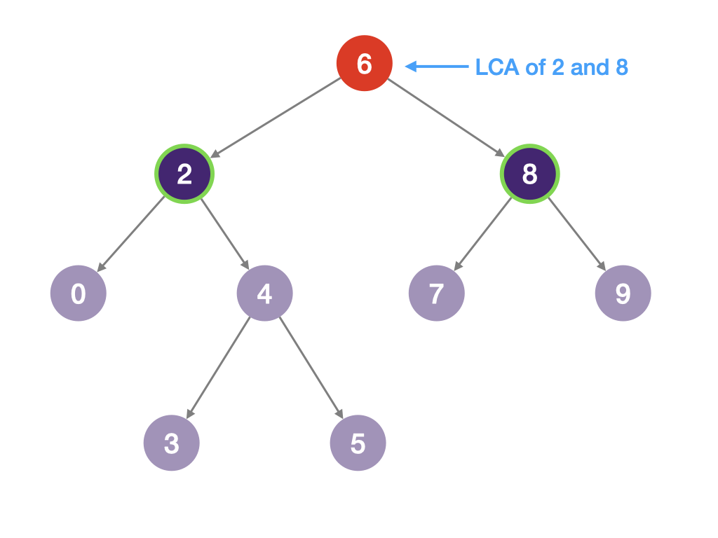
This video provides an excellent walkthrough of this exact logic.

Python Code Snippet: Iterative LCA for BST

class TreeNode:
    def __init__(self, val=0, left=None, right=None):
        self.val = val
        self.left = left
        self.right = right

def lowestCommonAncestor_BST(root: 'TreeNode', p: 'TreeNode', q: 'TreeNode') -> 'TreeNode':
    current = root
    
    while current:
        # If both p and q are greater than current, LCA must be in the right subtree.
        if p.val > current.val and q.val > current.val:
            current = current.right
        # If both p and q are less than current, LCA must be in the left subtree.
        elif p.val < current.val and q.val < current.val:
            current = current.left
        # Otherwise, we've found the split point: the LCA.
        # This is the case where one is on the left and one is on the right,
        # or one of the nodes is the current node.
        else:
            return current
    return None # Should not be reached if p and q are in the tree

Concept 3: LCA in a General Binary Tree (The Recursive Search)

What if the tree isn't a BST? We can no longer use node values to guide our search. We have to search the entire tree. The standard approach is a recursive Depth-First Search (DFS).

Technical Explanation

The core idea is to define a recursive function that returns "evidence" from each subtree. The function findLCA(node, p, q) will return:

• The node itself if it finds p or q.
• The LCA if it was found within its subtree.
• None if it finds neither p nor q in its subtree.

At any given root, the logic is as follows:

1. Base Case: If root is None, or if root is p or q, return root.
2. Recursive Step: Recursively call findLCA on the left and right children:
   • left_result = findLCA(root.left, p, q)
   • right_result = findLCA(root.right, p, q)
3. Synthesize Results:
   • If left_result and right_result are both non-null, it means p was found in one subtree and q in the other. Therefore, the current root is the LCA. Return root.
   • If only one of them is non-null (e.g., left_result), it means either both p and q are in the left subtree, or just one of them is. In either case, we propagate the non-null result upwards: return left_result (or right_result).
   • If both are null, neither node was found in this subtree. Return None.

The time complexity is $O(N)$ because we must visit every node in the worst case. The space complexity is $O(H)$ due to the recursion stack, which is $O(N)$ in the worst case (a skewed tree).

Python Code Snippet: Recursive LCA for Binary Tree

def lowestCommonAncestor_BT(root: 'TreeNode', p: 'TreeNode', q: 'TreeNode') -> 'TreeNode':
    # Base case: if we've reached the end of a branch, or found p or q.
    if not root or root == p or root == q:
        return root

    # Recursively search the left and right subtrees.
    left_result = lowestCommonAncestor_BT(root.left, p, q)
    right_result = lowestCommonAncestor_BT(root.right, p, q)

    # If the recursive calls on both subtrees returned a non-null node,
    # it means p and q were found in different subtrees of the current 'root'.
    # Therefore, the current 'root' is their LCA.
    if left_result and right_result:
        return root

    # If only one of the subtrees returned a node, it means either:
    # 1. Both p and q are in that subtree.
    # 2. Only one of p or q has been found so far.
    # In either case, we propagate that result upwards.
    # If both were null, this correctly returns null.
    return left_result or right_result

Concept 4: Under the Hood: Tracing the Recursive Calls

The recursive solution for a general binary tree is elegant but can be tricky to visualize. Let's trace the call stack to solidify your understanding.

Technical Explanation

The magic of the algorithm lies in how information propagates up the call stack. A node doesn't need to know what its children found, only that they found something.

Consider this execution flow:

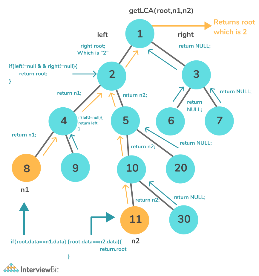
Let's break down the logic from the algo.monster article you read: return root if left and right else (left or right).

• if left and right: This is the "LCA found" case. The current root is the pivot point.
• else (left or right): This is the "propagate evidence" case.
  • If left is a node and right is None, this evaluates to left.
  • If left is None and right is a node, this evaluates to right.
  • If both are None, this evaluates to None.
    This single line elegantly handles three distinct outcomes.

Real-world System Example: The DOM Tree

In web development, the Document Object Model (DOM) is a tree structure representing an HTML page. A common task in a framework like React is to find the smallest container element that encloses two different components that were updated. This is exactly an LCA problem. When React needs to re-render efficiently, it finds the smallest common subtree (rooted at the LCA) that needs to be updated, rather than re-rendering the entire page.

Concept 5: The Parent Pointer Variant (An Elite Interview Twist)

Top companies like Google and Meta often add twists to standard problems to test adaptability. A common variant for LCA is: "What if each node has a parent pointer?"

Technical Explanation

If you have parent pointers, you can solve this problem without recursion and without starting from the root. It becomes a list intersection problem.

Imagine you have two nodes, p and q. The paths from each node up to the root form two singly-linked lists that are guaranteed to intersect (at the LCA and all its ancestors). The problem is now "find the intersection point of two linked lists."

1. Calculate Depths: Find the depths of p and q.
2. Align Pointers: Move the pointer of the deeper node up by the difference in depths. Now both pointers are at the same level.
3. Traverse Upward: Move both pointers up one step at a time, simultaneously. The first node they meet at is the LCA.

This approach is often more efficient if the nodes are very deep in a large tree, as you don't need to visit the entire tree. The time complexity is $O(H)$ and space complexity is $O(1)$.

A more elegant version of this avoids calculating depth explicitly.

This variant tests a different set of skills: recognizing that a problem can be transformed into another well-known pattern (list intersection) and applying the corresponding optimal algorithm.

Conclusion

Today you've explored the Lowest Common Ancestor problem from multiple angles, a requirement for elite-level interviews. You've seen how a problem's constraints (BST vs. general tree) completely change the optimal solution.

Key Takeaways:

• LCA Definition: The lowest node that has both p and q as descendants, where a node is a descendant of itself.
• BST Approach: An efficient iterative $O(\log N)$ solution is possible by using the BST property to navigate towards the "split point."
• Binary Tree Approach: A recursive $O(N)$ DFS is required. The key is propagating "evidence" of found nodes up the call stack. The node that receives evidence from both its left and right children is the LCA.
• Recursive Logic: The expression return root if left and right else (left or right) is a powerful and concise way to implement the recursive logic.
• Parent Pointer Variant: If parent pointers exist, the problem transforms into finding the intersection of two linked lists, solvable in $O(H)$ time and $O(1)$ space.

Preview of the Next Lesson

Having covered several core tree structures (BT, BST, Heaps), our next lesson introduces a specialized tree optimized for string and prefix-based operations: the Trie (or prefix tree). You will learn to implement a Trie and apply it to solve classic problems like autocomplete and dictionary searches. This is a crucial data structure for many applications dealing with textual data.