Quicksort: In-Place Partitioning and Performance Analysis

1. The Core Idea: Divide and Conquer through Partitioning

Quicksort's strategy is elegant and follows the Divide and Conquer pattern perfectly:

1. Divide: Pick an element from the array, called the pivot. Rearrange the array so that all elements smaller than the pivot are to its left, and all elements greater than the pivot are to its right. The pivot is now in its final, sorted position. This process is called partitioning.
2. Conquer: Recursively apply Quicksort to the sub-array of smaller elements and the sub-array of larger elements.
3. Combine: Nothing to do here! Because the partitioning is done "in-place" (within the original array), the array is already sorted once the recursive calls finish.

To see this process in action, let's watch an excellent conceptual overview.

After partitioning, the pivot is "locked in" its final sorted place. The problem is now reduced to sorting the two smaller, independent sub-arrays on either side of it.

2. In-Place Partitioning Schemes

The "magic" of Quicksort happens in the partitioning step. A key feature is that it's an in-place algorithm, meaning it sorts the data within the existing array structure, requiring only a small, constant amount of extra memory for variables (and the recursive call stack, which we'll discuss later).

As a developer, it's useful to know that there isn't just one way to partition. Two of the most famous schemes are the Lomuto and Hoare partition schemes. The method shown in the Abdul Bari video is a variation of the Hoare scheme.

Let's explore the pseudocode for these schemes to understand their mechanics.

So which one is better? It's a trade-off, which is a common theme in software architecture.

With a partitioning scheme chosen, the main Quicksort algorithm is surprisingly simple. It's a recursive function that calls the partition method and then calls itself on the two resulting sub-arrays.

Here is the pseudocode for the main recursive function, which uses a generic PARTITION function.

QUICK_SORT(A, low, high)
  if low < high
    p := PARTITION(A, low, high)
    QUICK_SORT(A, low, p - 1)
    QUICK_SORT(A, p + 1, high)

(Note: The exact recursive calls might be QUICK_SORT(A, low, p) for the left part with some partition schemes like the one in Abdul Bari's video, depending on what the partition index p represents).

For a complete, runnable example in Java that you can examine, check out the implementation from Sedgewick and Wayne's "Algorithms, 4th Edition". You can find the code for partitioning and the recursive sort on slides 6 and 7 of the lecture notes (Resource ID LINK).

3. Performance Analysis: When Quicksort is Quick (and when it's not)

This is the most critical part of our lesson. Why is an algorithm with "quick" in its name sometimes slow? It all comes down to how well the pivot divides the array.

Best and Average Case: O(n log n)

The ideal scenario is that the pivot is always the median element, splitting the array into two equal halves.

• The array of size $n$ is split into two arrays of size $n/2$.
• Each of those is split into two of size $n/4$, and so on.
• The number of times you can halve the array is ${\log }_{2}n$. This is the depth of the recursion.
• At each level of recursion, the partitioning process involves scanning all $n$ elements.
• Total work: $O(n)$ work per level $\times$ $O(\log n)$ levels = $O(n\log n)$.

Crucially, even if the split isn't perfectly 50/50, as long as it's reasonably balanced (e.g., 25/75), the complexity remains $O(n\log n)$. This is why the average-case performance on random data is excellent.

Worst Case: O(n²)

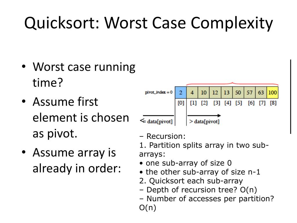
The worst case occurs when the partitioning is maximally unbalanced. This happens when the pivot is always the smallest or largest element in the sub-array.

• The array of size $n$ is split into one sub-array of size 0 and another of size $n-1$.
• The recursion depth becomes $n$.
• At each level, we still do roughly $O(n)$ work.
• Total work: $O(n)$ work per level $\times$ $O(n)$ levels = $O(n^2)$.

This disastrous scenario most commonly occurs when trying to sort an already sorted or reverse-sorted array, if you are naively picking the first or last element as the pivot.

Let's watch a video that ties these concepts together.

As the video mentions, these practical improvements are essential. In most production-quality Quicksort implementations, you won't find a naive pivot selection. Instead, strategies like:

• Randomized Pivot: Pick a random element as the pivot. This makes it statistically very unlikely that you'll consistently pick bad pivots.
• Median-of-Three: Look at the first, middle, and last elements of the sub-array, and choose the median of those three as the pivot. This is a good heuristic to avoid the worst-case on sorted or nearly-sorted data.

Conclusion

You have now completed a deep dive into Quicksort, one of the most important algorithms in computer science. You've gone beyond just knowing what it is to understanding how it works and, more importantly, why it performs the way it does.

Key Takeaways:

• Quicksort is an efficient, in-place sorting algorithm based on the Divide and Conquer paradigm.
• The core of the algorithm is the partition step, for which multiple in-place schemes like Lomuto and Hoare exist.
• Performance is fundamentally tied to pivot selection.
  • Average/Best Case: $O(n\log n)$ with balanced partitions.
  • Worst Case: $O(n^2)$ with unbalanced partitions, often triggered by sorted data and naive pivot choice.
• Practical implementations avoid the worst case by using smarter pivot strategies like randomization or median-of-three.

Preview of the Next Module:

This lesson concludes our module on Algorithmic Design Paradigms. You've built a solid foundation by exploring and contrasting Divide and Conquer, Greedy algorithms, and Dynamic Programming.

In our next module, Dynamic Programming in Practice, we will transition from theory to application. The first lesson will guide you to implement a dynamic programming solution using memoization (the top-down approach), directly applying the DP concepts we introduced earlier.