Level-Order Traversal with a Queue

1. What is Level-Order Traversal?

Level-order traversal means visiting all nodes at a given depth before moving on to the next depth. Within each level, nodes are visited from left to right.

For example, given this tree:

      F
     / \
    D   J
   / \ / \
  B  E G  K
 /     \
A       I

The level-order traversal would be: F, D, J, B, E, G, K, A, I.

This animated GIF provides an excellent visual intuition for the process.

A simple recursive approach, which works well for depth-first traversals, is not a natural fit here. How would you "jump" from the rightmost node of one level to the leftmost node of the next? This is where we need a data structure to help us keep track of the nodes we need to visit next.

2. The Algorithm: Breadth-First Search with a Queue

The perfect tool for this job is a queue. By using a queue, we can process nodes in the exact order we discover them. This technique is a specific application of a fundamental graph algorithm called Breadth-First Search (BFS). Since a tree is a type of graph, BFS is the ideal pattern for a level-by-level traversal.

The core logic is as follows:

1. Initialize a queue and add the root node to it.
2. While the queue is not empty:
   a. Dequeue a node (let's call it current).
   b. Process current (e.g., print its value or add it to a list).
   c. Enqueue the left child of current, if it exists.
   d. Enqueue the right child of current, if it exists.

The following video provides a clear, step-by-step walkthrough of this process.

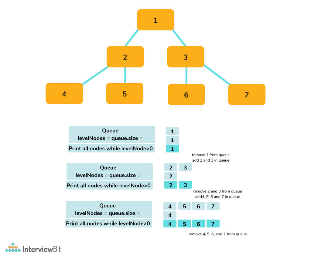
To reinforce this, the image below provides a static, step-by-step breakdown you can study at your own pace.

      10
     /  \
    5    15
   / \    \
  2   7    20

3. Implementation and a Common Variation

Now, let's translate this logic into an implementation. A frequent requirement is not just to print the nodes in order, but to return them grouped by level, like [[3], [9, 20], [15, 7]]. This requires a small but clever tweak to our algorithm.

The Algo.monster article provides an excellent, concise explanation of the algorithm and this level-grouping technique.

As the article explains, the enhanced algorithm is:

1. Initialize a queue with the root node and a list for the final answer.
2. While the queue is not empty:
   a. Get the current size of the queue. This is the number of nodes in the current level.
   b. Create a temporary list for the current level's values.
   c. Loop size times:
   i. Dequeue a node.
   ii. Add its value to the temporary level list.
   iii. Enqueue its children (if they exist).
   d. Add the temporary level list to the final answer list.
3. Return the final answer list.

With your full-stack background, you can appreciate seeing this implemented in different languages. The following resource provides complete code examples.

4. Complexity Analysis

A key part of the architectural mindset is understanding the performance implications of the algorithms you choose. Let's analyze the level-order traversal.

• Time Complexity: $O(n)$
  This is because every node in the tree is visited (enqueued and dequeued) exactly once. The work done for each node—processing its value and enqueuing its children—is constant time. Therefore, the total time is directly proportional to the number of nodes, $n$.

• Space Complexity: $O(W)$, where $W$ is the maximum width of the tree.
  The space is dominated by the queue. At any point, the maximum number of nodes the queue will hold is the number of nodes in the tree's widest level.

  • Worst Case: For a complete and perfectly balanced binary tree, the last level contains approximately $n/2$ nodes. In this case, the space complexity becomes $O(n)$.
  • Best Case: For a skewed tree (essentially a linked list), the width is always 1. The space complexity is $O(1)$.

The final section of the first video provides a good summary of this analysis.

Conclusion

In this lesson, you've mastered a fundamental tree traversal algorithm. By leveraging a queue, you can efficiently visit a tree's nodes breadth-first, which has applications in areas like shortest path finding in unweighted graphs (which we'll see later) and serialization/deserialization of trees.

Key Takeaways:

• Level-order traversal visits nodes level by level, left-to-right, implementing a Breadth-First Search (BFS) on the tree.
• A queue is the essential data structure for this algorithm, as its FIFO property ensures nodes are processed in the correct order.
• A common implementation pattern involves using a nested loop and the queue's size to group nodes by their level.
• The time complexity is always $O(n)$, as each node is processed once.
• The space complexity is $O(W)$, where $W$ is the maximum width of the tree, making it $O(n)$ in the worst case for a wide, balanced tree.

You now have a solid command of both depth-first (recursive) and breadth-first (iterative with a queue) traversal methods.

In our next lesson, we will transition from implementing specific algorithms to a higher-level design task: "Apply a hash table or a BST to solve a problem, justifying the choice of data structure." This moves us firmly into architectural thinking, where selecting the right tool for the job is as important as knowing how to use it.