Bulk-to-Boundary Propagators and CFT Two-Point Functions

1. The Strategy: From On-Shell Action to Correlators

Let's recall the master formula from the last lesson, which connects the CFT generating functional of connected correlators, $W_{CFT}[\phi_0]$, to the on-shell supergravity action, $S_{SUGRA, on-shell}[\phi_0]$:

where $\phi_0(x)$ is the boundary value of the bulk field $\phi(x,z)$, which acts as a source for the operator $O(x)$.

From this, we can extract correlation functions via functional differentiation. The two-point function is given by:

This gives us a clear computational procedure:

1. Solve the classical equation of motion for the bulk field $\phi$ for an arbitrary source $\phi_0$ at the boundary.
2. Substitute this on-shell solution back into the classical action.
3. Evaluate the action, which, as we'll see, reduces to a boundary term.
4. Differentiate the resulting on-shell action twice with respect to the source to obtain the two-point function.

2. Physical Intuition: The Geodesic Approximation

Before diving into the full field theory calculation, let's build a physical picture. Consider a very heavy bulk particle, which corresponds to a CFT operator with a very large conformal dimension $\Delta \gg 1$. In this limit, the quantum fluctuations of the particle's path are suppressed, and its dynamics are dominated by the classical path—a geodesic in the AdS spacetime.

The two-point function $\langle O(x_1) O(x_2) \rangle$ can be thought of as the amplitude for creating an excitation at boundary point $x_1$ and annihilating it at $x_2$. In the bulk, this corresponds to a particle propagating from $x_1$ to $x_2$ along the boundary. The shortest path for the particle is a geodesic arc through the bulk that connects these two boundary points.

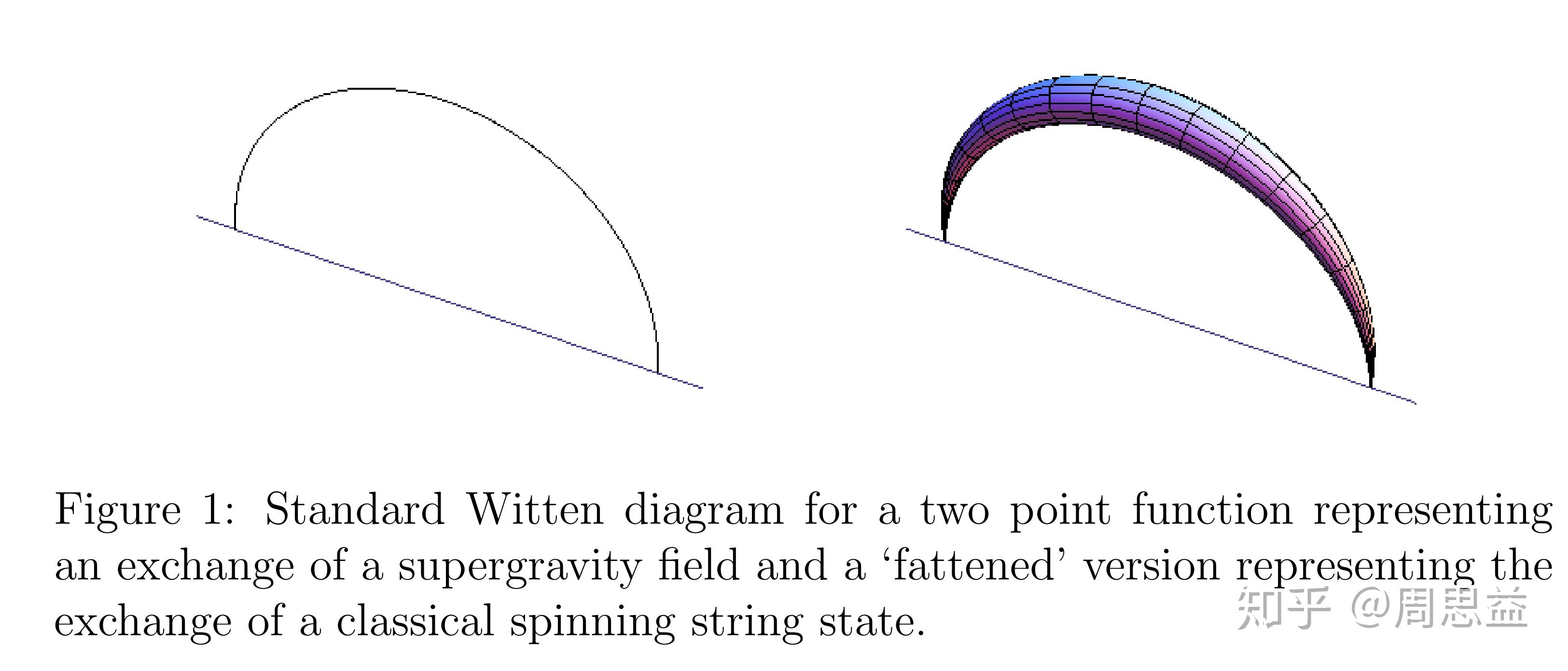
The classical action for a massive particle is simply its mass times the length of its worldline. So, the leading contribution to the two-point function in this limit is:

where $\gamma$ is the geodesic connecting $x_1$ and $x_2$.

As Maldacena explains, the proper length of the geodesic is infinite because the boundary is infinitely far away. By introducing a cutoff at $z=\epsilon$, the regulated length is found to be:

Plugging this into the action and using the large-dimension limit of our mass-dimension formula, $m \approx \Delta/L$, we get:

Ignoring the cutoff-dependent prefactor, which can be absorbed into the operator normalization, we recover the celebrated result from conformal symmetry:

This geodesic approximation gives us the right answer and a powerful intuition, but it's only valid for large $\Delta$. Now, let's perform the full field theory calculation that holds for any $\Delta$.

3. The General Calculation: Bulk-to-Boundary Propagators

To solve the system for any source $\phi_0(x)$, we introduce a crucial tool: the bulk-to-boundary propagator, denoted $K_\Delta(x, z; y)$. This is the solution to the bulk Klein-Gordon equation that corresponds to a delta-function source at a single point $y$ on the boundary. In Poincaré coordinates, it has the form:

With this Green's function, the general solution for an arbitrary source $\phi_0(y)$ is given by superposition:

The bulk-to-boundary propagator can be found by solving the wave equation or, more elegantly, by applying an AdS isometry to a simpler solution. The result is remarkably simple:

where $c_\Delta$ is a normalization constant. You can verify that this function solves the scalar wave equation in AdS and has the correct scaling properties.

With the classical solution in hand, we can now compute the on-shell action.

Let's summarize the key steps of the calculation presented in the notes:

1. Action and Variational Principle: The standard bulk action for a scalar field needs to be supplemented with a specific boundary term (the Gibbons-Hawking-York term, generalized here) to make the variational problem well-posed when we fix the value of the field at the boundary.

   $$S={\int }_{AdS}\sqrt{g}\left[\frac{1}{2}(\nabla \varphi {)}^2+\frac{1}{2}{m}^2{\varphi }^2\right]+\text{boundary term}$$

2. Integration by Parts: Using the equation of motion, $(\nabla^2 - m^2)\phi = 0$, the bulk part of the action vanishes on-shell. The entire on-shell action is then given by a surface integral at the boundary $z \to 0$.

   $$S_{on-shell}\propto {\int }_{z=ϵ}{d}^{d}x\sqrt{\gamma }\varphi n^{\mu }{\partial }_{\mu }\varphi$$

   where $\gamma$ is the induced metric on the boundary slice and $n^\mu$ is the outward-pointing normal vector. In Poincaré coordinates, this simplifies to an integral involving $\phi \partial_z \phi$.

3. Evaluating the Action: We now substitute our classical solution, $\phi(x,z) = \int d^dy , K_\Delta(x,z;y)\phi_0(y)$, into this boundary integral. After a careful calculation involving taking the $z \to 0$ limit, the action becomes a quadratic functional of the source $\phi_0$:

   $$S_{on-shell}=-\frac{1}{2}\int d^{d}x\int d^{d}y{\varphi }_0(x){\varphi }_0(y)\frac{C}{|x-y{|}^{2\Delta }}$$

   where $C$ is a constant related to $c_\Delta$.

4. Extracting the Correlator: Finally, we take two functional derivatives with respect to the source $\phi_0$ to get the two-point function:

   $$⟨O(x_1)O(x_2)⟩\approx -\frac{{\delta }^2{S}_{on-shell}}{\delta {\varphi }_0(x_1)\delta {\varphi }_0(x_2)}=\frac{C}{|x_1-x_2{|}^{2\Delta }}$$

This result is the triumphant outcome of our calculation. We have derived the form of a CFT two-point function entirely from a classical field theory calculation in one higher dimension.

4. Witten Diagrams and Generalizations

The calculation we just performed can be generalized. If we include interaction terms like $\lambda \phi^3$ in the bulk action, we can compute three-point functions $\langle O(x)O(y)O(z) \rangle$. The calculation involves three bulk-to-boundary propagators meeting at an interaction vertex in the bulk, which we then integrate over all possible bulk positions.

This perturbative expansion of CFT correlators in terms of bulk interactions is elegantly captured by Witten diagrams, which are essentially Feynman diagrams for the bulk theory. The external legs of these diagrams, however, don't represent particles but rather end on the boundary, representing the operator insertions. Our two-point function calculation corresponds to the simplest Witten diagram: a single line (the bulk propagator) connecting two points on the boundary.

Conclusion

In this lesson, we have made the holographic dictionary a powerful computational tool. By applying the GKPW prescription in the classical gravity limit, we successfully derived the form of a CFT two-point function from the on-shell action of its dual bulk field.

Key Takeaways:

• The two-point function in the CFT can be computed from the second functional derivative of the on-shell bulk action with respect to the boundary source.
• The bulk-to-boundary propagator is the fundamental building block for constructing the classical bulk solution for any given boundary source.
• The on-shell action for a free field reduces to a boundary integral, which, when evaluated, yields a non-local term quadratic in the boundary source. This non-local term is precisely the generating functional for the two-point function.
• The entire procedure confirms the form $\langle O(x)O(y) \rangle \propto |x-y|^{-2\Delta}$, where $\Delta$ is related to the bulk mass by the formula we derived in the previous lesson.
• This method can be visualized with Witten diagrams and generalized to compute higher-point correlation functions by including interaction vertices in the bulk.

Next Lesson Preview:

So far, our discussion has been fairly general. The most famous and powerful version of the AdS/CFT correspondence, relating $\mathcal{N}=4$ Super Yang-Mills theory to Type IIB string theory on $AdS_5 \times S^5$, is an exact duality, not just an approximation. This exactness is deeply rooted in the enormous amount of symmetry present. In our final lesson of this module, we will explore the critical role that superconformal symmetry plays in constraining the theory and making such a precise and powerful statement of equivalence possible.