Model Comparison Experiment Design

Welcome to the final lesson of our first module, where we've been taking an architect's view of a machine learning project. We've journeyed from framing a business problem to diagnosing model fit, and most recently, to establishing a crucial performance baseline. You'll recall that a baseline provides the "floor" for performance, giving context to our metrics and justifying the pursuit of more complex models.

Now, with a baseline in place, we arrive at the culminating step of this initial design phase: selecting a champion model. This isn't a matter of guesswork or simply picking the model with the highest score after a single run. From an architectural standpoint, model selection must be a deliberate, structured, and defensible process. This lesson will equip you to design a formal model comparison experiment. We'll move beyond ad-hoc evaluations to a rigorous methodology that allows you to confidently select the best algorithm for your production system.

The Model Selection Workflow

At a high level, the process of evaluating and choosing a model follows a clear sequence of steps. This workflow ensures that you are methodical in your approach, which is critical for reproducibility and sound decision-making.

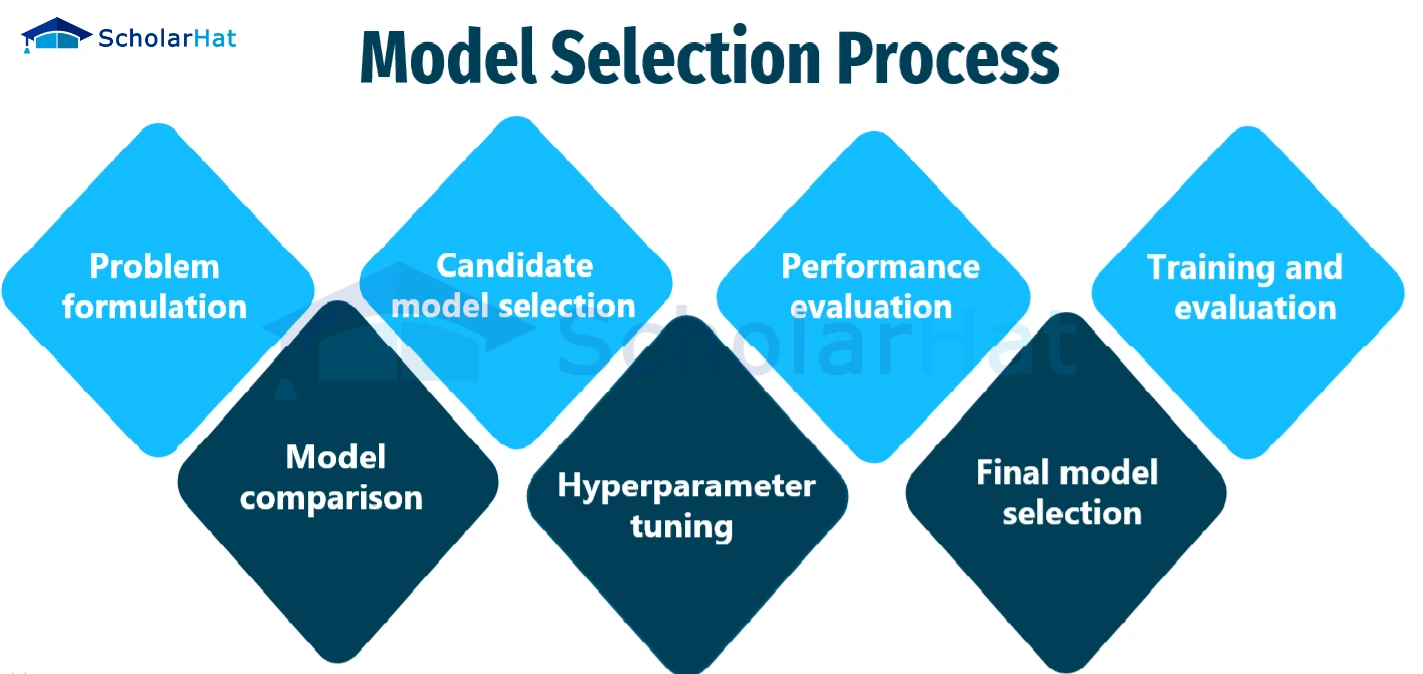
This flowchart illustrates the key stages in a machine learning model selection process. We will focus on the latter stages: candidate selection, performance evaluation, comparison, and final selection, all of which form the core of a model comparison experiment.

As you can see, model comparison isn't a single action but a sub-process involving evaluation and tuning. Our goal in this lesson is to formalize this process.

Anatomy of a Machine Learning Experiment

To treat model comparison with the necessary rigor, we should frame it as a scientific experiment. This involves defining a clear structure, which ensures your results are valid, reproducible, and can be communicated clearly to stakeholders. A well-designed experiment moves your conclusion from "Model A seems better" to "Model A is statistically superior to Models B and C under these specific conditions, and here is the evidence."

The following presentation slides offer an excellent framework for designing such experiments.

[PDF] Designing Effective Machine Learning Experiments - NC State ISE

This document from North Carolina State University provides a concise yet comprehensive guide to the principles of experimental design in machine learning. It aligns perfectly with the structured approach an architect should take.

Please read the following sections: Start with the slides titled "What is an ML Experiment?" and "Why is Experiment Design Important?" to understand the rationale. Next, study the 8-step process outlined across the slides titled "The Experiment Design Process". Pay close attention to the definitions of independent, dependent, and controlled variables. Finally, review the slide "Important Considerations" and its best practices. Notice how "Start with a simple baseline" directly connects to our previous lesson.

Let's summarize the key components of our model comparison experiment, based on this framework:

Objective: To determine which candidate algorithm (e.g., Logistic Regression, Random Forest, k-NN) yields the best performance for our specific problem and chosen metric (e.g., F1-score for a classification task).
Hypothesis: The null hypothesis ( $H_{0}$ ) is that all candidate models have equal performance. Our experiment aims to gather enough evidence to reject this hypothesis and identify a superior model.
Independent Variable: The machine learning algorithm/model being tested.
Dependent Variable: The performance metric(s) we measure (e.g., mean cross-validated accuracy, F1-score, AUC).
Controlled Variables: To ensure a fair comparison, everything else must be held constant. This is where our work from previous lessons pays off.
- Dataset: All models are trained and evaluated on the same data.
- Validation Protocol: All models are evaluated using the exact same k-fold cross-validation splits. This is non-negotiable.
- Preprocessing: All models are preceded by the same data preprocessing steps, enforced by our scikit-learn Pipeline.

Implementing a Fair Comparison

With the experimental design defined, implementation becomes straightforward. You'll select a slate of candidate models and evaluate each one using the exact same procedure.

A good practice is to select a diverse set of candidates that represent different algorithmic families:

Linear models: Logistic Regression (for classification) or Linear Regression (for regression). They are fast, interpretable, and extend our simple baseline.
Instance-based models: k-Nearest Neighbors (k-NN).
Tree-based ensembles: Random Forest or Gradient Boosting. These are often high-performers.

The scikit-learn Pipeline object makes it incredibly easy to swap out the final estimator while keeping the preprocessing steps identical. The following video provides a clear, practical demonstration of this exact workflow.

Scikit-Learn Model Pipeline Tutorial

This tutorial by Greg Hogg demonstrates how to use scikit-learn Pipelines to compare different regression models on the same task.

Watch the segment from this point, where the instructor first trains a k-Nearest Neighbors model and then seamlessly replaces it with a Random Forest model within the same pipeline structure to compare their performance. This is the core workflow for a model comparison experiment.

To generalize this, you can create a loop that iterates over a dictionary of models, runs cross_val_score on each, and stores the results for comparison.

Here's how you might structure this in code:

import numpy as np
from sklearn.model_selection import KFold, cross_val_score
from sklearn.pipeline import make_pipeline
from sklearn.preprocessing import StandardScaler
from sklearn.linear_model import LogisticRegression
from sklearn.neighbors import KNeighborsClassifier
from sklearn.ensemble import RandomForestClassifier
from sklearn.datasets import make_classification




# 1. Create a synthetic dataset
X, y = make_classification(n_samples=1000, n_features=20, n_informative=10, n_redundant=5, random_state=42)




# 2. Define the controlled variables
# The same CV object ensures identical splits for all models
cv_splitter = KFold(n_splits=10, shuffle=True, random_state=42)



# The same preprocessing pipeline
preprocessor = StandardScaler()




# 3. Define the independent variables (candidate models)
models = {
    "Logistic Regression": LogisticRegression(max_iter=1000),
    "k-NN": KNeighborsClassifier(n_neighbors=5),
    "Random Forest": RandomForestClassifier(random_state=42)
}




# 4. Run the experiment
results = {}
for name, model in models.items():



    # Create the full pipeline for the current model
    pipeline = make_pipeline(preprocessor, model)
    



    # Evaluate the model using the same CV splits
    scores = cross_val_score(pipeline, X, y, cv=cv_splitter, scoring='accuracy', n_jobs=-1)
    



    # Store the results
    results[name] = scores
    print(f"{name}: Mean Accuracy = {np.mean(scores):.4f} (Std = {np.std(scores):.4f})")




# Expected Output (will vary slightly):
# Logistic Regression: Mean Accuracy = 0.8460 (Std = 0.0341)
# k-NN: Mean Accuracy = 0.8840 (Std = 0.0276)
# Random Forest: Mean Accuracy = 0.9380 (Std = 0.0213)

Based on this output, Random Forest appears to be the winner. But is a mean accuracy of 93.8% definitively better than k-NN's 88.4%? And if the difference were smaller, say 93.8% vs 93.6%, could you confidently state that one is superior?

Beyond Averages: The Role of Statistical Significance

Merely comparing the mean scores is often not enough, especially when the differences are small. The scores we calculated are estimates based on a finite sample of data. If we were to draw a different sample, the scores would change. Statistical hypothesis tests allow us to determine the probability that the observed performance difference is real and not just a result of random chance in our data sample.

As an architect, you need to ensure your team's claims of model superiority are robust. Knowing which statistical tests to apply provides the necessary evidence to make a defensible decision. Sebastian Raschka's article is an authoritative guide on this topic.

Model evaluation, model selection, and algorithm selection ...

This article provides a deep dive into the statistical tests used for comparing machine learning models and algorithms. It's a key resource for moving from informal comparison to rigorous analysis.

Please read the following sections: Comparing Two Models: Read McNemar's Test. This is a classic test for comparing two classifiers on the same test set. Focus on understanding the 2x2 contingency table that compares their predictions (correct vs. incorrect), as this is the core intuition. Comparing Multiple Models: Read Multiple Hypotheses Testing to understand the problem of running too many pairwise tests. Then, read about Cochran’s Q Test, which acts as an "omnibus" test to see if any model in a group performs differently. The standard procedure is to run Cochran's Q first, and if it's significant, run pairwise McNemar tests with a correction. Comparing Algorithms (A More Robust Approach): The tests above compare specific trained models. A more robust approach compares the learning algorithms themselves by accounting for variance in the training data. Read about Dietterich’s 5x2-Fold Cross-Validated Paired t-Test. This is a highly regarded standard for algorithm comparison. The Gold Standard: Finally, read the section on Nested Cross-Validation. This is considered a best practice for getting an unbiased performance estimate, especially when hyperparameter tuning is involved (which we'll cover in Module 5). It prevents information from the model selection process from "leaking" into the final performance evaluation. Skim the summary figure in the Conclusions section for a great overview of when to use which test.

The key takeaway is not that you must perform these calculations by hand, but that a formal process exists to validate your choice. For an architect, being able to say "We selected Random Forest because it showed a statistically significant performance lift over other candidates, confirmed with a 5x2cv paired t-test" is far more powerful than saying "Random Forest had the highest score."

The Architect's Decision Matrix

The winning model from our experiment is the champion based on a single metric. However, the final choice for a production system involves a broader set of criteria. As the system architect, you must balance performance with operational and business constraints.

Your final decision matrix should include:

Predictive Performance: The primary metric from your experiment (e.g., Accuracy, F1, RMSE).
Inference Latency: How long does the model take to make a single prediction? This is critical for real-time applications. A complex deep learning model might be slightly more accurate but too slow for production use.
Training Time & Cost: How long does it take to train the model? A model that takes days to train on expensive hardware might not be feasible for a system that requires frequent retraining.
Interpretability: Can you explain why the model made a particular prediction? For regulatory or debugging purposes, a simpler model like Logistic Regression might be preferred over a "black box" like a large ensemble.
Maintenance & Dependencies: How complex is the model to deploy and maintain? Does it have exotic dependencies that complicate your production environment?

Conclusion

In this lesson, we've formalized the process of model selection, elevating it from a simple leaderboard comparison to a structured experiment. This approach provides the rigor and defensibility required when making key architectural decisions for a production ML system.

Here are the main takeaways:

Design a Formal Experiment: Frame model selection with a clear objective, hypothesis, and controlled variables to ensure your comparison is fair and reproducible.
Use a Consistent Evaluation Protocol: Leverage scikit-learn Pipelines and a fixed KFold object to ensure all candidate models are evaluated on the exact same footing.
Validate with Statistical Tests: Go beyond comparing mean scores. Use statistical tests like McNemar's or the 5x2cv paired t-test to confirm that performance differences are statistically significant and not just due to random chance.
Consider the Full Picture: The "best" model is a balance of predictive performance and practical, operational constraints like latency, training cost, and interpretability.

This lesson concludes our first module. We have established a complete, high-level workflow for a machine learning project, from problem framing to final model selection. You are now equipped with the architect's view of the end-to-end process.

In our next module, "Data Preprocessing and Feature Engineering," we will zoom in on the critical first step of this workflow: transforming raw data into high-quality features suitable for modeling. We will explore techniques for handling missing values, encoding categorical data, feature scaling, and more—the essential building blocks for the preprocessing steps we've used in our pipelines.

Recommended resources