Sliding Window Counter: Beyond Fixed Windows

Your learning outcome for this lesson:

By the end of this lesson, you will be able to describe the sliding window counter algorithm and explain how it addresses the limitations of the fixed window approach.

1. The Core Idea: From Fixed Windows to Sliding Windows

The fundamental problem with the Fixed Window Counter is the hard reset at the window boundary. The algorithm has no memory of what happened just before the new window started. The solution, logically, is to create a window that "slides" forward in time, continuously considering the most recent time interval.

Instead of asking, "How many requests has this client made in the current minute?", a sliding window algorithm asks, "How many requests has this client made in the last 60 seconds?"

This subtle change in perspective is key. A burst of requests spanning a minute boundary (e.g., from 10:30:59 to 10:31:01) will now be counted within the same rolling 60-second window, preventing the client from exceeding the limit.

While the concept is simple, the implementation requires a more clever approach than just a single counter. Let's explore two common ways this algorithm is realized.

2. Two Flavors of the Sliding Window Counter

The "Sliding Window Counter" is best understood as a category of algorithms that approximate a true sliding window. We'll look at two primary implementations, moving from a simple approximation to a more precise and practical one that you'll use in your project.

Approach A: The Weighted Counter Approximation

This approach is a direct and clever enhancement of the Fixed Window algorithm. It's less memory-intensive and simpler to reason about. It operates by keeping track of two counters: one for the previous window and one for the current window.

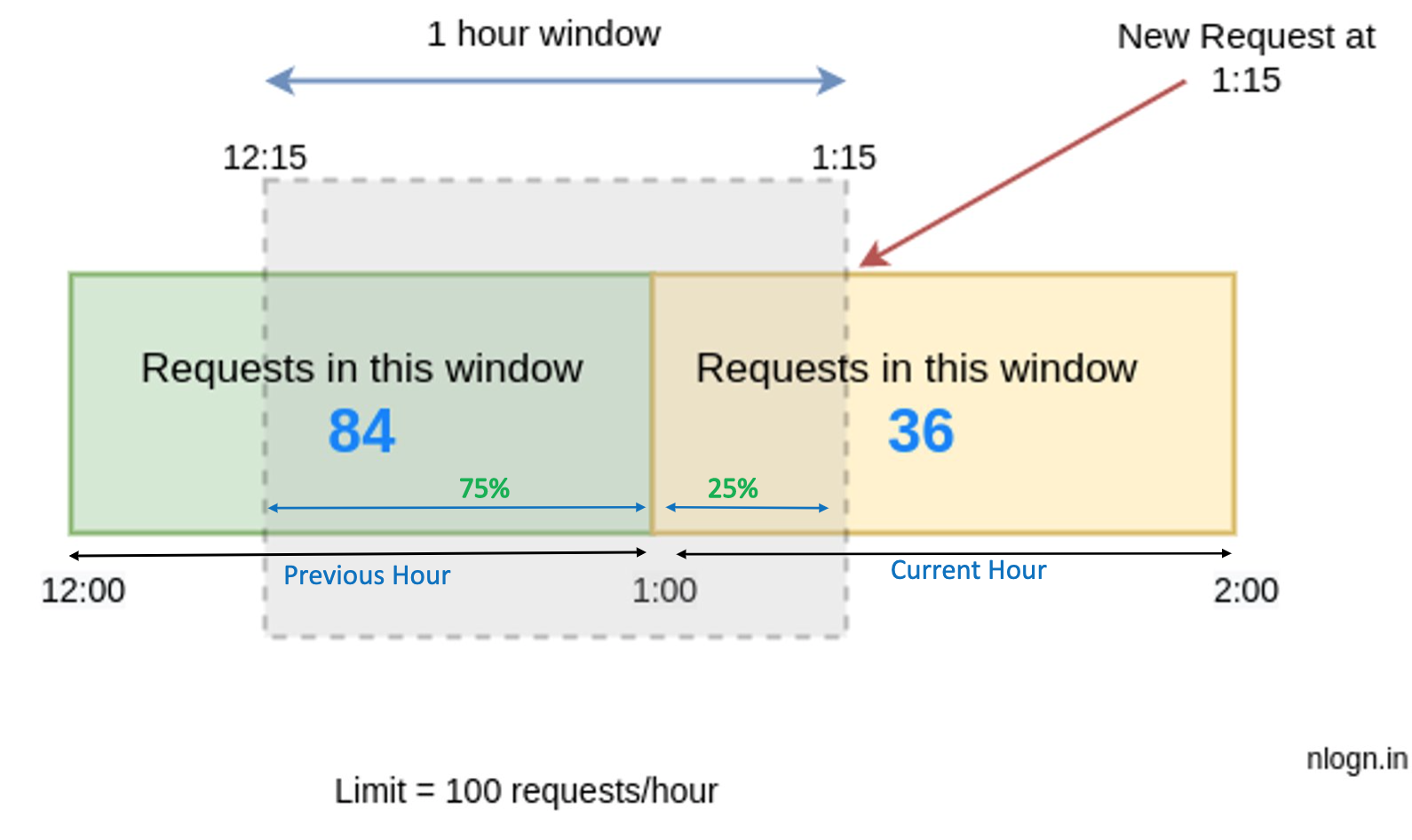
When a new request arrives, it estimates the count in the true sliding window by taking a weighted sum:

estimated_count = (percentage_of_previous_window * previous_window_count) + current_window_count

The "percentage of previous window" is the portion of the last window that still falls within the current sliding frame.

Let's make this concrete with an example.

This image from the article visually represents the calculation:

Trade-offs of this approach:

• Pro: It's very efficient, requiring only two counters per client.
• Con: It assumes requests were evenly distributed throughout the previous window, which is often not true. A burst at the beginning of the previous window might have already "slid" out of view, but the algorithm would still count a fraction of it, leading to a potentially inaccurate estimate.

Approach B: The Sub-Interval (or Bucketing) Counter

This is a more accurate and widely used implementation, especially in distributed systems. It's the approach we'll favor for your project as it maps perfectly to data structures available in Redis.

The idea is to divide the main time window (e.g., 60 seconds) into smaller, more granular sub-intervals or "buckets" (e.g., six 10-second buckets). The system maintains a counter for each bucket.

When a request arrives:

1. The algorithm identifies the current bucket (e.g., based on timestamp / 10).
2. The counter for that bucket is incremented.
3. To check the rate, the algorithm sums the counts of all buckets that fall within the last 60 seconds.
4. As time moves forward, older buckets naturally fall outside the 60-second sliding window and are no longer included in the sum.

This method provides a much smoother and more accurate rolling average of the request rate.

To reinforce this, the same concepts are also covered in a companion article.

This sub-interval approach strikes an excellent balance. It's far more accurate than the simple weighted counter and far more memory-efficient than the "Sliding Window Log" algorithm, which we'll discuss next.

3. Differentiating from Sliding Window Log

You may also encounter the Sliding Window Log algorithm. It's important to understand the difference.

• Sliding Window Log:

  • Stores a timestamp for every single request in a log (e.g., a sorted set or list).
  • To check the rate, it removes all timestamps older than the window duration and then counts the remaining entries.
  • Pro: It's perfectly accurate. There is no approximation.
  • Con: The memory and computational costs are very high, as the log can grow very large, making it impractical for high-traffic APIs.

• Sliding Window Counter (Sub-Interval):

  • Groups requests into buckets and only stores a counter per bucket.
  • Pro: Much lower memory usage and computational cost.
  • Con: It's an approximation, but usually a very good one. The accuracy depends on the granularity of the buckets (smaller buckets = more accuracy, more memory).

The Sliding Window Counter is the pragmatic choice for most real-world systems, offering a fantastic trade-off between accuracy and performance.

Key Takeaways

• The Sliding Window Counter algorithm solves the boundary burst problem of the Fixed Window by considering a rolling time frame, not a static one.
• The Weighted Counter is a simple implementation that uses counters from the previous and current windows. It's efficient but less accurate.
• The Sub-Interval (Bucketing) Counter is a more accurate and practical approach. It divides the window into smaller buckets, providing a smoother rate calculation. This is the method you will be implementing with Redis.
• The Sliding Window Counter is a practical compromise, offering most of the accuracy of the Sliding Window Log algorithm without its prohibitive memory and computational costs.

Next Steps

We have now covered two counter-based algorithms. You understand the simple-but-flawed Fixed Window and the more robust Sliding Window.

In the next lesson, we will shift our perspective entirely and look at the Token Bucket algorithm. Instead of counting requests, this algorithm deals with pre-allocated capacity and a refill rate. It's another production-grade algorithm with different performance characteristics, and understanding it is essential for building a versatile rate limiter.