Good to see you again. Last lesson established the key local object behind optimization: the gradient. For the squared-error linear model
you derived one gradient component for the intercept and one for the weight. A negative component meant that increasing that parameter would locally reduce loss; a positive component meant decreasing it would locally reduce loss.
This lesson takes the next, operational step: use the gradient to change all parameters once, evaluate whether the change helped, and interpret the role of the learning rate. This is the basic training loop underlying much of machine learning, from linear and logistic models to neural networks.
From a gradient to a parameter update
Let the parameter vector be
and let be the loss computed on the training data. Gradient descent updates the parameters by
where:
- is the iteration number;
- is the gradient evaluated at the current parameters;
- is the learning rate;
- is the step calculated from the gradient.
The minus sign is the essential feature. The gradient points in the direction of steepest local increase in loss, so subtracting it moves in the direction of steepest local decrease.
For the two parameters separately, the rule is:
All gradient components must be calculated from the same old parameter setting, and the updates happen simultaneously. Do not update , recompute the model, and then update using that partially updated model. That would be a different algorithm.
The four-step gradient-descent diagram below captures the wider loop. This lesson focuses closely on the transition from steps 2 to 3: turning a computed gradient into one controlled move.
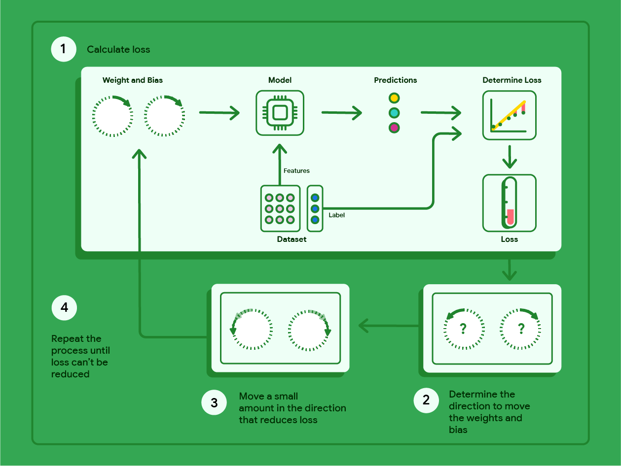
Linear regression: Gradient descent | Machine Learning
Read the numerical walkthrough in Google's Machine Learning Crash Course. It shows the same update rule applied to a small linear-regression dataset, including how slopes for weight and bias become new parameter values.
In the expanded mathematical walkthrough after Figure 11, begin where the model is initialized at zero. Read the full numerical update. Track three quantities separately: the current parameters, the derivatives at those parameters, and the learning-rate-scaled update. Google uses ordinary MSE rather than the half-MSE convention used in the previous lesson, so its displayed derivatives are twice as large for otherwise equivalent models.
One complete update by hand
Continue with the two-observation example from the previous lesson:
The model is
and the loss is the half mean squared error:
At the current parameter setting,
the predictions are and , while the residuals are and . Thus the current loss is
From the previous lesson, the gradient at this point is
Choose a learning rate of
The gradient-descent step is
Add this step to the old parameter vector:
Equivalently, applying the update component by component:
Interpret the signs
Both partial derivatives were negative:
A negative derivative says that a small increase in that parameter should reduce loss locally. Subtracting a negative gradient component correctly increases both and .
The updated model is
Its predictions are:
The new residuals are therefore and , giving
The loss fell from to . This confirms that this particular update improved the model's fit to these training observations.
The larger update to does not mean the feature is inherently more important. It says only that, at this parameter setting and this feature scale, the loss was more sensitive to a change in than to an equally sized change in .
The learning rate controls caution, not direction
The gradient determines a direction. The learning rate determines how far to move in that direction.
A small learning rate takes cautious steps:
This may reduce loss reliably, but it can require many iterations before parameters get close to a minimum.
A larger learning rate moves more aggressively. It may reduce loss faster, but it can overshoot the minimum. In our example, try using
with the same initial gradient:
The resulting predictions are and , which are much too high for the target values and . The loss becomes
So this larger step makes the loss worse than the original loss of .
This does not contradict the fact that the negative gradient is a descent direction. It is a local statement: a sufficiently small move in the negative-gradient direction reduces loss to first order. A large move can jump across the valley and land at a higher-loss location.
Gradient Descent, Step-by-Step
Watch StatQuest's “Gradient Descent, Step-by-Step” for a compact visual treatment of updating an intercept and slope together. It reinforces the important point that a two-parameter update is one move on a loss surface, not two unrelated one-dimensional procedures.
Watch the joint update. Focus on the sequence: choose current intercept and slope, evaluate both derivatives there, multiply each by one learning rate, and form the next pair of parameters simultaneously. Notice the warning that a learning rate suitable for one parameterization or dataset may be unsuitable for another.
Loss scaling changes the numerical learning rate
You may encounter either of these squared-error objectives:
They have the same minimizing parameters because one is exactly twice the other:
But their gradients differ:
That is why Google’s walkthrough can report derivatives that look different from yours even when the underlying model and data are equivalent. If a loss is multiplied by , then a learning rate should be divided by to produce the same parameter step.
The lesson is practical: never interpret a learning rate in isolation. Its useful scale depends on:
- the loss definition;
- the number and scale of features;
- the current local shape of the loss surface;
- whether the loss is averaged over observations.
For example, multiplying a numerical feature by can greatly change the associated weight gradient. This is one reason feature scaling becomes important in gradient-based model fitting.
Express the update in matrix form
For a linear model with an intercept, create a design matrix whose first column is all ones:
and write the parameter vector and outcomes as
Then the prediction vector is
For the half-MSE loss, the gradient is
The update is simply
This is the version worth recognizing in real code: matrix multiplication calculates the predictions and accumulates every parameter's derivative efficiently.
import numpy as np

# First column is the intercept feature.
X = np.array([
    [1.0, 1.0],
    [1.0, 3.0]
])

y = np.array([2.0, 5.0])
theta = np.array([0.0, 1.0])  # [b, w]
learning_rate = 0.1

def half_mse_loss(theta, X, y):
    errors = X @ theta - y
    return 0.5 * np.mean(errors ** 2)

def gradient(theta, X, y):
    errors = X @ theta - y
    return X.T @ errors / len(y)

old_loss = half_mse_loss(theta, X, y)
grad = gradient(theta, X, y)

# The right-hand side uses only the old theta and its gradient.
new_theta = theta - learning_rate * grad
new_loss = half_mse_loss(new_theta, X, y)

print("Old parameters:", theta)
print("Gradient:", grad)
print("New parameters:", new_theta)
print("Old loss:", old_loss)
print("New loss:", new_loss)
The key outputs should be approximately:
Gradient: [-1.5 -3.5]
New parameters: [0.15 1.35]
Old loss: 1.25
New loss: 0.2225
A compact audit for any hand calculation or implementation is:
- State the parameter order.
- Calculate predictions and loss using the current parameters.
- Calculate the gradient in that same parameter order.
- Compute the step .
- Apply the whole vector update simultaneously.
- Recompute the loss at the new parameters as a diagnostic.
For a one-step calculation, an improved loss is useful evidence that the sign, gradient, and learning-rate scale are sensible. It is not a guarantee that every future step will reduce loss, nor does a decreasing training loss establish that the model will generalize well to new data.
Key takeaways
Gradient descent changes parameters using
The negative gradient supplies a local direction of loss reduction. The learning rate controls the step magnitude: too small can be slow, while too large can overshoot and increase loss.
For the example starting at , the gradient
and learning rate produce the simultaneous update
which lowers the half-MSE from to .
This completes the optimization foundations module. Next, the course turns to probability foundations, beginning with how marginal, joint, and conditional probabilities are computed from a probability table.